Download
1 / 44
440 likes | 453 Views
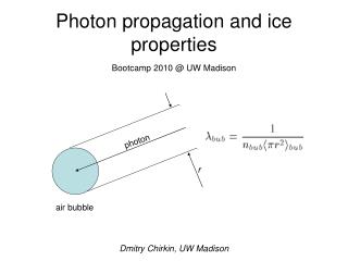
Photon propagation and ice properties. Bootcamp 2011 @ UW Madison. photon. r. air bubble. Dmitry Chirkin, UW Madison. Propagation in diffusive regime. absorption. scattering. r 2 =A . r 1 < r 2 >=<A . r 1 >= t < r 1 >. q. Photon propagation approximations. cascades near: far:

E N D
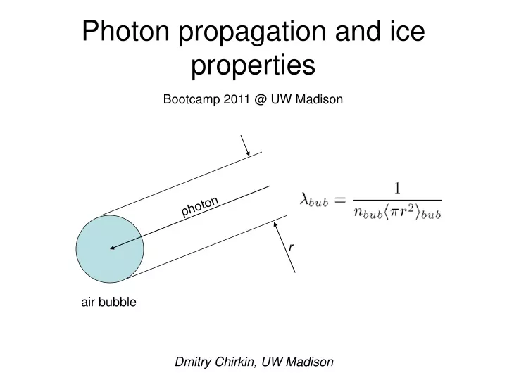
Photon propagation and ice properties Bootcamp 2011 @ UW Madison photon r air bubble Dmitry Chirkin, UW Madison
Propagation in diffusive regime absorption scattering r2=A.r1 <r2>=<A.r1>=t<r1> q
Photon propagation approximations • cascades • near: • far: • combined: • diffusive formula actually also gives correct limit at small distances but is difficult to compute (see icecube/201102007) • muons • near: • far: • combined:
cascades ~1/r2 far numerical merged small angle nearby ~1/r exp(-r/lp) ppc simulation
muons ~1/r far merged nearby ~1/r1/2 exp(-r/lp) ppc simulation
Mie scattering theory Continuity in E, H: boudary conditions in Maxwell equations e-i|k||r| r e-ikr+iwt
Mie scattering theory • Analytical solution! • However: • Solved for spherical particles • Need to know the properties of dust particles: • refractive index (Re and Im) • radii distributions
Mie scattering theory Dust concentrations have been measured elsewhere in Antarctica: the “dust core” data
Scattering function: approximation • Mie scattering • - General case for scattering off particles
Scattering and Absorption of Light Source is blurred scattering absorption Source is dimmer a = inverse absorption length (1/λabs) b = inverse scattering length (1/λsca)
Measuring Scattering & Absorption • Install light sources in the ice • Use light sensors to: • - Measure how long it takes • for light to travel through ice • - Measure how much light is delayed • - Measure how much light does not • arrive • Use different wavelengths • Do above at many different depths scattered absorbed
Embedded light sourcesin AMANDA isotropic source (YAG laser) cosq source (N2 lasers, blue LEDs) tilted cosqsource (UV flashers) 45°
Timing fits to pulsed data Make MC timing distributions at grid points in le-la space At each grid point, calculate c2 of comparison between data and MC timing distribution (allow for arbitrary tshift) Fit paraboloid to c2 grid ►Scattering: le±se ►Absorption: la±sa ►Correlation: r ►Fit quality: c2min
Fluence fits to DC data • In diffusive regime: • N(d) 1/dexp(-d/lprop) • lprop = sqrt(lale/3) • c = 1/lprop dust d1 d2 No Monte Carlo! DC source log(Nd) c1 slope = c c2 c1 d
Light scattering in the ice dusty bands bubbles shrinking with depth
3-component model of absorption Ice extremely transparent between 200 nm and 500 nm Absorption determined by dust concentration in this range Wavelength dependence of dust absorption follows power law
A 6-parameter Plug-n-Play Ice Model scattering id=301 Power law: l-a be(l,d) be(400,d) id=302 A = 6954 ±973 B = 6618 ±71 D = 71.4±12.2 E = 2.57 ±0.58 a = 0.90 ±0.03 k = 1.08 ± 0.01 Linear correlation with dust: CMdust= D·be(400) + E absorption 3-component model: CMdustl-k+ Ae-B/l a(l,d) T(d) id=303 Temperature correction: Da = 0.01a DT
AHA model Additionally Heterogeneous Absorption: deconvolve the smearing effect
Is this model perfect? Individually fitted for each pair: best possible fit Points at same depth not consistent with each other! Fits systematically off
Is this model perfect? When replaced with the average, the data/simulation agreement will not be as good From ice paper Averaged scattering and absorption Measured properties not consistent with the average! Deconvolving procedure is unaware of this and is using the averages as input
SPICE: South Pole Ice model • Start with the bulk ice of reasonable scattering and absorption • At each step of the minimizer compare the simulation of all flasher events at all depths to the available data set • do this for many ice models, varying the properties of one layer at a time select the best one at each step • converge to a solution!
SPICE Mie [mi:] Dmitry Chirkin, UW Madison
Simplified Mie Scattering Also known as the Liu scattering function Introduced by Jon Miller Single radius particles, described better as smaller angles by SAM
Dependence on g=<cos(q)> and fSAM g=<cos(q)> fSAM 0.8 0 0.9 0 0.95 0 0.9 0.3 0.9 0.5 0.9 1.0 flashing 63-50 64-50
Dependence on <cosq> and fSL cascades muons
Verification with toy simulation Input table Simulated 60 x 250 events Reconstructed table with 10 event/flasher 250 event/flasher In the dust peak
Correlation with dust logger With 10 events/flasher, 250 in dust peak With 250 events/flasher everywhere
Plots for individual flashers SPICE Mie AHA
Plots for CORSIKA/data SPICE Mie AHA
Global scaling to ice parameters Minimum is in the same place with both likelihoods!
IceCube in-ice calibration devices 3 Standard candles 56880 Flashers 7 dust logs
Correlation with dust logger data (from Ryan Bay) effective scattering coefficient Scaling to the location of hole 50 fitted detector region
Improvement in simulation by Anne Schukraft by Sean Grullon Downward-going CORSIKA simulation Up-going muon neutrino simulation
Photon tracking with tables • First, run photonics to fill space with photons, tabulate the result • Create such tables for nominal light sources: cascade and uniform half-muon • Simulate photon propagation by looking up photon density in tabulated distributions • Table generation is slow • Simulation suffers from a wide range of binning artifacts • Simulation is also slow! (most time is spent loading the tables)
PTD Photons propagated through ice with homogeneous prop. Uses average scattering No intrinsic layering: each OM sees homogeneous ice, different OMs may see different ice Fewer tables Faster Approximations Photonics Photons propagated through ice with varying properties All wavelength dependencies included Layering of ice itself: each OM sees real ice layers More tables Slower Detailed Light propagation codes: two approaches (2000)
PTD vs. photonics: layering Bulk PTD Layered PTD photonics 2 3 2 1 2 3 2 1 2 3 2 average ice type 1 type 2 type 3 “real” ice
Direct photon tracking with PPC photon propagation code • simulates all photons without the need of parameterization tables • using Henyey-Greenstein scattering function with <cos q>=0.8 • using tabulated (in 10 m depth slices) layered ice structure • employing 6-parameter ice model to extrapolate in wavelength • transparent folding of acceptance and efficiencies • Slow execution on a CPU: needs to insert and propagate all photons • Quite fast on a GPU (graphics processing unit): is used to build the SPICE model and is possible to simulate detector response in real time.