Download
1 / 30
300 likes | 372 Views
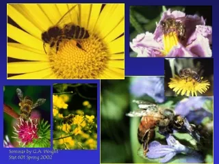
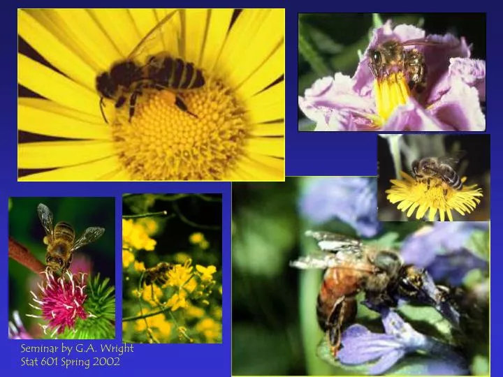
Seminar by G.A. Wright Stat 601 Spring 2002. While flying slowly in a patch of flowers, a bee may encounter an inflorescence every 0.14 s (Chittka et al., 1999). How do bees recognize floral perfumes among different flowers?. What characteristics of a floral perfume do they remember?.

E N D
Seminar by G.A. Wright Stat 601 Spring 2002
While flying slowly in a patch of flowers, a bee may encounter an inflorescence every 0.14 s (Chittka et al., 1999)
How do bees recognize floral perfumes among different flowers? What characteristics of a floral perfume do they remember?
Characteristics of floral perfumes: • often, made up of many (100 +) odor compounds • some compounds are present at high concentrations, others are present at low concentrations • (sometimes several orders of magnitude difference)
How do floral perfumes vary among individual flowers? • temporal variation: diurnally and developmentally • inter-plant variation: individuals, varieties, species, and families
Variation in major scent components of snapdragon varieties N. Dudareva and N. Gorenstein, Purdue Univ.
Three parameters of a floral perfume that may affect the learning and memory of honeybees: 1) Types of compounds present 2) Variation in the intensity of the components 3) Intensity of each component relative to the intensity of the perfume
Methods • Two types of 3-component mixtures: • “Similar” compounds: • hexanol, heptanol, and octanol • “Dissimilar” compounds: • hexanol, geraniol, and octanone • Two concentrations: • Low: 0.0002 M • High: 2.0 M A 3-component mixture where one odor concentration is fixed and the others are allowed to vary randomly at low or high conc. produces 22 = 4 possible mixture combinations.
Three Experiments 1) Constancy of a single odor component 2) Average concentration of each component versus variation in individual components 3) Variability of all components versus mixture osmolality
Experiment I Constant odor at the low concentration Two concentrations used to make odor mixtures: low and high
Constant odor at the high concentration Two concentrations used to make odor mixtures: low and high
Using eitherthe similar odors or the dissimilar odors, each component of the mixture was systematically held constant Bees were trained over 16 trials with either: - constant odor at low or - constant odor at high eg. dissimilar mixture: hexanol = constant odor Then, they were tested with each odor component of the mixture at either: - low concentration or - high concentration eg. dissimilar mixture: tested with hexanol, geraniol, and octanone
Proboscis extension by honeybees during associative conditioning Trial 1 Trial 2 Trial 3 Odor Sucrose Proboscis extension
mixture type constant odor test concentration low low high Similar high low high low low high Dissimilar high low high
Used PROC LOGISTIC in SAS for analysis of data: Variables entered in the analysis: 1) Level of the constant odor (coded: 0,1) 2) Level of the test components (coded: 0, 1) 3) Identity of the test components (coded: 0, 1) 4) Response variable: 0 = no response, 1 = response The analysis was separated by mixture type (similar and dissimilar)
Experiment I Similar SAS Output for logistic regression Parameter DF Estimate SE Chi-Square Pr > ChiSq Exp(Est) Intercept 1 0.4055 0.1757 5.3266 0.0210 1.500 mixlev 1 2.0959 0.3729 31.5902 <.0001 8.133 tstlev 1 -1.0655 0.2527 17.7822 <.0001 0.345 mixlev*tstlev 1 -2.5753 0.4618 31.0968 <.0001 0.076
Experiment I Dissimilar SAS Output for logistic regression Parameter DF Estimate Error Chi-Square Pr > ChiSq Exp(Est) Intercept 1 1.0442 0.2625 15.8182 <.0001 2.841 mixlev 1 1.1816 0.4654 6.4461 0.0111 3.259 tstlev 1 -0.6369 0.3558 3.2051 0.0734 0.529 tstodre 1 0.4446 0.3280 1.8373 0.1753 1.560 mixlev*tstodre 1 1.0923 0.4252 6.5980 0.0102 2.981 mixlev*tstlev 1 -1.8121 0.5079 12.7287 0.0004 0.163 tstlev*tstodre 1 -1.3244 0.4249 9.7167 0.0018 0.266
Conclusions of Experiment I Similar odors: Sensory system adaptive gain control: If training (constant) odor is high and test odor is low, the response to all odors decreases, and visa versa Dissimilar odors: Gain Control: same as for similar odors Constant odor preferred: If training (constant) odor the same as the test odorant, then the response to constant odor increases Interaction between: test odorant identity and odorant intensity Suggestion of an interaction between variation and intensity
Experiment II: Average concentration of each component vs. variation in individual components Using eitherthe similar odors or the dissimilar odors, Bees were trained over 16 trials with either: - a mixture with all odorants at a constant middle (0.02 M) - or only one odor at a constant middle (0.02 M), and the others at either low or high (thus, average middle) Then, they were tested with each odor component of the mixture at the low concentration
Used PROC LOGISTIC in SAS for analysis of data: Variables entered in the analysis: 1) Experiment type (coded: 0,1) 2) Identity of the test components (coded: 0, 1) 3) Response variable: 0 = no response, 1 = response The analysis was separated by mixture type (similar and dissimilar)
Experiment II Similar Dissimilar SAS Output for logistic regression Parameter DF Estimate SE Chi-Square Pr > ChiSq Exp(Est) Intercept 1 1.3863 0.5590 6.1497 0.0131 4.000 tstodre 1 -0.7672 0.6499 1.3936 0.2378 0.464 exp 1 -1.7540 0.7075 6.1465 0.0132 0.173 tstodre*exp 1 0.6723 0.8404 0.6400 0.4237 1.959 Similar Dissimilar Parameter DF Estimate SE Chi-Square Pr > ChiSq Exp(Est) Intercept 1 -0.6190 0.4688 1.7433 0.1867 0.538 exp 1 1.1045 0.6494 2.8928 0.0890 3.018 tstodre 1 0.9213 0.5675 2.6352 0.1045 2.512 exp*tstodre 1 -1.6944 0.7882 4.6218 0.0316 0.184
Conclusions of Experiment II When tested with the low concentration components: Similar odors: If the training odorants are at a constant concentration, the response to the test odorant increases Dissimilar odors: Constant odor preferred: If one of the odorants is constant in the mixture, the response to the constant odorant increases Suggestion of an interaction between variation and intensity and mixture type
Experiment III: Variability of all components versus mixture osmolality Using eitherthe similar odors or the dissimilar odors, Bees were trained over 16 trials with either: - a mixture with all odorants at a constant (0.7 M), producing a mixture with osmolality = 2.1 M - a mixture with all odorants at varying concentrations producing a mixture with osmolality = 2.0 M - a mixture with all odorants at varying concentrations producing a mixture with osmolality = 0.03 M Then, they were tested with each odor component of the mixture at the low concentration
Used PROC LOGISTIC in SAS for analysis of data: Variables entered in the analysis: 1) Variability (high or low) (coded: 0,1) 2) Mixture osmolality (coded: 0, 1) 3) Response variable: 0 = no response, 1 = response The analysis was separated by mixture type (similar and dissimilar)
Experiment III Similar Dissimilar SAS Output for logistic regression Parameter DF Estimate SE Chi-Square Pr > ChiSq Exp(Est) Intercept 1 1.5755 0.3950 15.9125 <.0001 4.833 mixlev 1 1.3802 0.2205 39.1896 <.0001 3.976 cv 1 -2.3977 0.3469 47.7793 <.0001 0.091 mixtype 1 -0.6612 0.2089 10.0177 0.0016 0.516
Conclusions of Experiment III • Similar and Dissimilar odors: • The magnitude of the response to the low concentration components is a measurable function of: • 1) Variation in the concentration of the components • 2) Osmolality of the mixture
Conclusions: • Types of compounds present affect generalization to constant • components 2) Variation in the intensity of the components increases generalization to the components 3) The intensity of the perfume produces an adaptive gain control which affects the ability of bees to detect low level components
Photo courtesy of NOVA Acknowledgements:Thanks to: Brian Smith, Amanda Mosier, Beth Skinner, Cindy Ford, Joe Latshaw, Sue Cobey, Natalia Dudareva for the snapdragons and volatiles data. Funded by NIH.