Download
1 / 19

E N D
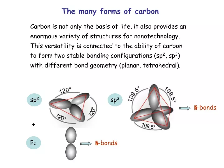
The many forms of carbon Carbon is not only the basis of life, it also provides an enormous variety of structures for nanotechnology. This versatility is connected to the ability of carbon to form two stable bonding configurations (sp2, sp3) with different bond geometry (planar, tetrahedral). sp2 sp3 -bonds + pz -bonds
* orbital - + - and - bonds -bond: orbital -bond: -orbital (bonding) *-orbital (antibonding)
Diamond3D sp3 Graphite,Graphene (= single sheet)2D sp2 Fullerene0D Nanotube1D
2D: Graphene, a single sheet of graphite A graphene sheet can be obtained simply by multiple peeling of graphite with sticky tape. A single sheet is visible to the naked eye. Graphene is very strong, has high electron mobility, and provides a transparent conductor with possible applications in displays and solar cells. The E(p) relation is linear instead of quadratic. 2010 Nobel Prize in Physics to Geim and Novoselov
Energy bands of graphite: sp2+pz M K Graphite is a semi-metal, where the density of states approaches zero at EFermi . The -bands touch EFermi only at the corners K of the Brillouin zone, while a free-electron band would form a Fermi circle. E sp2 * * pz EFermi px,y sp2 Brillouin zone s kx,y
Two-dimensional -bands of graphene E[eV] Empty EFermi Occupied K =0 M K Empty kx,y Occupied In two dimensions one has the quantum numbers E,kx,y. This plot of the energy bands shows E vertically and kx ,ky in the horizontal plane.
“Dirac cones” in graphene A special feature of the graphene -bands is the linear E(k) relationnear the six corners (K) of the Brillouin zone (instead of the parabolic relation for free electrons). In a three-dimensional E(kx,ky) plot one obtains cone-shaped energy band dispersions.
Topological Insulators A spin-polarized version of a “Dirac cone” occurs in “topological insulators”. These are insulators in the bulk and metals at the surface, because two surface bands bridge the bulk band gap. It is impossible topologically to remove the surface bands from the gap, because they are tied to the valence band on one side and to the conduc-tion band on the other. The metallic surface state bands have been measured by angle- and spin-resolved photoemission (see Lecture 19). Hasan and Kane, Rev. Mod. Phys.
1D: Carbon nanotubes Carbon nanotubes are grown using catalytic metal clusters (Ni, Co, Fe,…). (Lecture 7, Slide 7)
Indexing of Nanotubes Unwrap a nanotube into planar graphene zigzag m=0 armchair n=m chiral nm Circumference vector cr =ma1 + na2
Energy bands of carbon nanotubes: Quantization along the circumference Analogous to Bohr’s quantization condition an integer number of electron wavelengths needs to fit around the circumferenceof the nanotube. Otherwise the electron waves would interfere destructively. This leads to a discrete number of allowed wavelengths n and wave vectors kn=2/n along the circum-ference. Along the axis of the nanotube the electrons cane move freely. One gets a one-dimensional band for each quantized state. The kinetic energy p2/2m of the motion along the tube is added to the quantized energy level.
Scanning Tunneling Spectroscopy: dI/dV I/V 1 for V0 when metallic D(E) Density of states of a single nanotube Calculated Density of States D(E): Each peak shows the one-dimensional 1/E singularity at the band edge (see density of states in Lecture 13).
Distinguishing nanotubes with different n and m “Two-dimensional” spectroscopy: Measure both photon absorption (x-axis) and photon emission (y-axis).
0D: Fullerenes 1996 Nobel Prize in Chemistry to Curl, Kroto, Smalley Buckminster Fuller, father of the geodesic dome Buckminsterfullerene C60 has the same hexagon+pentagon pattern as a soccer ball. The pentagons (highlighted) provide the curvature. C60 solution in toluene
Symmetry Fullerenes with increasing sizeFewer pentagons produce less curvature.
Production of fullerenes Plasma generation of fullerenes in a Krätschmer-Huffman apparatus. Mass spectrum showing the different fullerenes generated.
Molecular orbitals of C60 The LUMO (lowest unoccupied molecular orbital) is located at the five-fold rings: The high symmetry of C60 leads to highly degenerate levels. i.e., many distinct wave functions have the same energy. Up to 6 electrons can be placed into the LUMO of a single C60 , making it a popular electron acceptor in organic solar cells.
C60 can be charged with up to 6 electrons The ability to take up that many electrons makes C60 a popular electron acceptor for molecular electronics, for example in organic solar cells.
* * photon LUMO, located at the strained five-fold rings Empty orbitals of fullerenes from X-ray absorption spectroscopy C1s core level