Download
1 / 25
260 likes | 391 Views
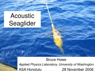
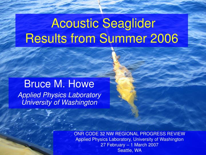
Acoustic Seaglider Results from Summer 2006. Bruce M. Howe Applied Physics Laboratory University of Washington. ONR CODE 32 NW REGIONAL PROGRESS REVIEW Applied Physics Laboratory, University of Washington 27 February – 1 March 2007 Seattle, WA. Goals and Outline.

E N D
Acoustic Seaglider Results from Summer 2006 Bruce M. Howe Applied Physics Laboratory University of Washington ONR CODE 32 NW REGIONAL PROGRESS REVIEW Applied Physics Laboratory, University of Washington 27 February – 1 March 2007 Seattle, WA
Goals and Outline • Develop and demonstrate the acoustic Seaglider in the persistent surveillance context: • As a communications gateway between subsurface platforms and land • To act as a general purpose acoustic receiver/tactical sensor for all signals and “noise”, with near-real time reporting of processed results • To provide oceanographic data • Review results from 3 field experiments • Discuss next steps
Acoustic Seaglider • ½ knot at ½ W • Up to 1000 m dives • > 6 months, 3000 km, 600 dives • Temperature, salinity and others • Now with hydrophone and acoustic modem Fumin Zhang
Acoustic Seaglider Operations – Summer 2006 Monterey Bay Kauai Philippine Sea Philippine Sea – SG022, 7/29/06-7/30/06, 1 day, 15 dives, low ARS band,CTD Monterey Bay – SG022, 8/15/06-8/21/06, 6 days, 61 dives, low ARS band,CTD SG023, 8/18/06-8/23/06, 5 days, 83 dives, low ARS band, CTD SG106, 8/12/06-8/18/06, 6 days, 131 dives, high + low ARS bands,CTD,mmodem Kauai - SG023, 8/31/06-10/8/06, 39 days, 143 dives, low ARS band, CTD
Monterey Bay 06:Positions where SG106 read mmodem FSK packets • Black circles: SG106 at surface after dive - no acomms received • Blue circles: dives where acomms commands logged • 106 sent FSK command to turn off the ARL-UT array • Most FSK came from ARL-UT or Gateway • Black +: dives after recording acomms logs ceased • 4-5 km ranges are evident ARL-UT bottom node 1 km Gateway Latitude Kelp Array First FSK packet at 2006.08.15:0857 (UTC) from unit ARL-UT to Gateway, Dive 22.
MB06: RXD receptions vs range and depth 0 m Depth Histograms of depths for RXD receptions SG106 ascending SG106 descending 100 m Counts 0 20 40 60 Counts 0 10 20 30 40 0 20 40 60 80 100 120 140 depth (m) 0 50 100 depth(m) 0 km Range 5 km
Modem performance: 1st 30 sec of dive 41 20 10 Missed packet 30 glider pump noise 25 Missed packet 20 Freq (kHz) telling UT-VS to talk to GB from kelp to GB 15 telling kelp to talk to GB 10 5 30 21:24:14 UTC ACOMMS band – 23-27kHz Reference band – 15-19kHz { 30 10 20 Time (s) PSD @ 8-10 sec Simple ACOMMS detector: ratio of energy in 23-27 kHz band to energy in 15-19 kHz band 0 5 10 15 20 25 30 35 kHz
Signals Example of Lubell source recorded at SG023 (dive 20 segment 2) MB06 LWAD Ship source, harmonics and reverb ~10 nm from ship Dive 13, file 2 Frequency Distant source Time (s) 150 0
NPAL / ATOC Kauai source • 260 W • M-sequence coded signals • 75 Hz, 35 Hz bandwidth • 28 ms peak • 27.28 s period • 2 hour transmissions, 1 per day Red segments = ARS recordings 79 30 DIVE 56 -example
} Example time series 1/75 Hz = 13.3 ms 10.8 ms 14.7 ms 13.0 ms } } } zoom PSD Kauai example Example PSD
(72.7195) Arrival times (72.8654) (72.9153) (73.4143) (72.282) Motion and Coherent gain • Single block 27.28 s • Peaks shift due to changing s/r range • Measured travel time changes • ~3.7 ms per block • Match glider kinematics • 0.204 m/s, 136 m horizontal, 33 m vertical, 12 minutes Relative travel time – 0.4 s Relative travel time – 0.4 s Relative travel time – 0.16 s • Doppler + stack: • from 35 to 44 dB • 9 dB of gain • vs theoretical gain 14 dB • Variation during 12 minutes Doppler Time – 12 minutes Time – 12 minutes
Animal sounds recorded on Seaglider ARS Monterey Bay, MB06 humpback Blue whale ‘D’ call Humpback (very close) Sea lions? birds Blue whale Blue whale ‘B’ call 3rd harmonic ~48 Hz Humpback @ 15 and 65 sec Blue @ 35 sec Sea Lions? @ 50 sec 1st harmonic ~16 Hz
ASG – Summer 2006 Summary • Demonstrated gateway capability – connecting subsurface platforms to shore via acoustic modem/satellite Iridium • Demonstrated acoustic receiver – man-made signals, whales, noise… with near-real time processed results • Potential – general ocean acoustics tool, tactical sensors, navigation/time node, data truck, marine mammal observing, tomography receiver, basin-scale thermometry, climate change, …
Next steps • Fall 07 – PLUSNet07 off La Jolla • Spring/summer – mini PLUSNet in Puget Sound + scouting mission off La Jolla • PLUS - Continuing development and field work • Communications: Modem integration and HFGW • Nexgen glider (payload, buoyancy, processing, …), • Tactical sensors – add directivity and gain • Mission management • Optimization: High currents, power, multiple gliders • Navigation and timing • Overall situational awareness • Integrating acoustics + nav into data assimilation – mobile acoustic tomography receiver
ONR Philippine Sea 2009 – Ocean acoustics deep water, QPE DRI (many) NASA: A Smart Sensor Web for Ocean Observation (APL, EE, JPL) NSF STC Coastal Margin Observation and Prediction (OHSU, OSU, UW) NSF ORION … Related Projects
Geoff Shilling Jason Gobat Craig Lee Russ Light Pete Sabin Rex Andrew Keith van Thiel Keith Magness Troy Swanson Tim McGinnis Mike Boyd Kate Stafford Sue Moore Robert Miyamoto Marc Stewart Jim Luby Neil Bogue Andrew White Jim Mercer Linda Buck Joe Wigton Fritz Stahr and the Seaglider Fabrication Center Lee Freitag and Matt Grund Tom Hoover, Jim Bellingham, et al Joe Curcio and the MIT kayaks Clay Spikes, Dave Porter, et al Yi Chao Pierre Lermusiaux ONR sponsorship Many helped! Skip Denny and the ANTS crew
Glider – Kayak interactions in Monterey Bay Kayaks pinging to glider Graphs by Alexander Bahr MITComputerScience &ArtificialIntelligenceLaboratory
Monterey Bay MB06 SG023 was allowed to drift on the surface for 2 extended periods during MB06 The resulting drifts were compared to surface current predictions from the HOPS model Leg 25 Leg 83 Current shear event experienced by glider but not captured by model nowcast forecast
Temperature, salinity, conductivity data usually available within 5 min of dive completion – example SG023 dive 46 Dive 46 temperature and salinity as plotted on IOP website
SG023 surface drifts Drift 2 shows a current shear event 80 Drift 2 78 recovered Drift 1 • Dives 55 and 83 followed by surface drift tests • Data compared to current prediction models
MB06 Acoustic Seaglider Accomplishments • Deploy and operate sensors in field • 428+ hours of dive time • 300+ dives (acomms, T, S, Depth, acoustics, surface currents, depth-avg currents) • Demonstrated Seaglider communications gateway capability • In-air – Iridium satellite • Sub-sea – acoustic modem at various depths and ranges • Passing NAFCON orders to remote kayak to prosecute target detected/reported by other kayaks (node of LBL navigation) • Turned bottom vector sensor array node on/off • Ambient sound • Active source emissions - Lubell source (for TL, propagation) • Marine mammals (blues, humpbacks, sea lions, …) • Ambient noise budget (ships, seismics, wind, rain, …) • Environmental data • Temperature and salinity into Harvard and JPL models • Depth averaged and surface currents • Bottom resting mode • Adaptive sampling
(72.7195) Arrival times (72.8654) (72.9153) (73.4143) (72.282) Coherent processing of M-sequence coded signals Relative travel time – 0.4 s Relative travel time – 27.28 s • Peaks in each block shift due to changing s/r range • Measured travel time changes • ~3.7 ms per 27.28 s block • Match glider kinematics • 0.0204 m/s, 136 m horizontally, 33 m vertically, in 12 minutes Relative travel time – 0.3 s