Download
1 / 18
180 likes | 271 Views
Virtual Product of Air Quality Demo Scripts. Liping Di, Peisheng Zhao Center for Spatial Information Science and Systems (CSISS) George Mason University ldi@gmu.edu. AQ Science Analysis-- Pollutant Sources, Transport Processes.

E N D
Virtual Product of Air Quality Demo Scripts Liping Di, Peisheng Zhao Center for Spatial Information Science and Systems (CSISS) George Mason University ldi@gmu.edu
AQ Science Analysis-- Pollutant Sources, Transport Processes • Purpose: To perform analysis regarding the sources and transport of air pollutants • Background: The pattern of air pollution is determined by the combined effects of emission sources, and by the interaction of transport, transformation and removal processes. The contribution of the various factors an be examined by simple analysis tools. • Analysis Tool: The analysis tool consists of display/browser of observed AQ data; source density, transport pattern and model simulations. • Usage: The analyst identifies the location of high pollution levels. Various AQ data are overlaid on top of emission density maps to see if the air resided over high pollutant emission regions. Based on satellite and model data, the analyst examines possible emissions from major fires. Given the location of high pollution values, model forecast transport simulations are displayed. • Services: Each data set is accessed through WMS/WCS/WFS, Portray, Overlaid, augmented by data wrappers and adopters. Chaining is executed at multiple servers to demonstrate interoperability. The tool is a special client. • Service Integration: A special client that allows data overlay, browsing as well as zoom and pan, in space and time.
Demo Specifics • Analyzing the sources and transport of pollutants from Canadian forest fires in June to USA. • The analyst needs to access to Air Quality Images, which is the integration of: • Surface visibility and meteorological conditions observed from AirNow and surface meteorological network. • Satellite observation (MODIS) • Political boundary • Date: • June 26, 2006; July 6, 2006 • By comparing the two images, the analyst will be able to find the source and transport of the pollutants • Geographic Region • United States and part of Canada • BBOX: -130, 24, -65, 52
Live Air Quality Demo-Step 1 • The analyst goes to OGC CSW catalog http://laits.gmu.edu:8099/cswquery-vdp/ • Search the air quality images for the specific date and geographic coverage. • The analyst finds there is no such a data product available
Live Air Quality Demo-Step 2 • The analyst is an expert on creating such a product through a geo-processing model. • The analyst goes to model designer : http://laits.gmu.edu/vdp/ and create the model using OGC service and data types schema with the help of the • The analyst registers the model as a virtual product in OGC CSW.
Live Air Quality Demo-Step 3 • The analyst goes to http://laits.gmu.edu:8099/cswquery-vdp/ again and search for air quality image for June 26 • The system responds with the availability of the image.
Live Air Quality Demo – Step 4 • The analyst retrieve the air quality image for June 26 through WCS interface. • The analyst repeats steps 3 and 4 again for July 6 image. • While waiting the system for producing the product on-live through the service chaining and execution • Explain what’s going on behind the scene through the following slides
Live Air Quality Demo Behind Scene – Workflow • The system converts the model to an executable workflow in BPEL by automatically plugging-in real services and data based on user’s specification. • Executes the workflow in BPELPower to generate the product on demand by using the distributed services • Accessing a point monitoring dataset (AIRNOW, SURF_MET ) • Aggregating from hourly to daily average • Portraying as a geoimage • Accessing satellite data • Overlaying the point and satellite data.
Behind the scene -- WCS Service • Accessing a point monitoring dataset AIRNOW.pmfine (DataFed WCS) http://webapps.datafed.net/ogc_EPA.wsfl?SERVICE=wcs&REQUEST=GetCoverage&VERSION=1.0.0&CRS=EPSG:4326&COVERAGE=AIRNOW.pmfine&FORMAT=dataset-schema& BBOX=-130,24,-65,52,0,0& TIME=2006-06-27T00:00:00Z/2006-06-27T15:00:00Z &WIDTH=1000&HEIGHT=600&DEPTH=99 Hourly to Daily
Behind the scene -- aggregation service 2. Aggregating AIRNOW.pmfine from hourly to daily average (DataFed Aggregator service) <TimeAggregate> <Table><TableRef>…</TableRef></Table> <Settings> <dataset_abbr>AIRNOW</dataset_abbr> <data_columns>pmfine</data_columns> <agg_oper>avg</agg_oper> <agg_limit>5000</agg_limit> <min_count>1</min_count> </Settings> </TimeAggregate>
Behind the scene—Render service 3. Portraying as a geoimage (DataFed Render service) <Render> <Table><TableRef>…</TableRef></Table> <Settings> <image_desc> <zoom><image_width>1000</image_width><image_height>600</image_height><lat_min>24</lat_min><lat_max>52</lat_max><lon_min>-130</lon_min><lon_max>-65</lon_max></zoom> <bgcolor>0xE1FFF0</bgcolor><image_format>image/png</image_format> </image_desc> <data_column>pmfine</data_column><scale_min>0</scale_min><scale_max>100</scale_max><sqrt>false</sqrt> <symbol><width>10</width><height>10</height><offset_x>0</offset_x><offset_y>0</offset_y><shape>circle</shape><num_of_sides>4</num_of_sides><baseline>false</baseline></symbol> <pen><width>0.5</width><style>solid</style><color>red</color></pen> <brush><style>solid</style><color>yellow</color></brush> <script>used.symbol.width=symbol.width*norm_param_value;used.symbol.height=symbol.height*norm_param_value;</script> </Settings> </Render>
Behind scene- Surface_Met WCS service 4. Accessing a point monitoring dataset SURF_MET.T (DataFed WCS) http://webapps.datafed.net/ogc_EPA.wsfl?SERVICE=wcs&REQUEST=GetCoverage&VERSION=1.0.0&CRS=EPSG:4326&COVERAGE=SURF_MET.T&FORMAT=dataset-schema& BBOX=-130,24,-65,52,0,0& TIME=2006-06-27T00:00:00Z/2006-06-27T15:00:00Z &WIDTH=1000&HEIGHT=600&DEPTH=99 Hourly to Daily
Behind the scene – Aggregator service for SURF_MET 5. Aggregating SURF_MET.T from hourly to daily average (DataFed Aggregator service) <TimeAggregate> <Table><TableRef>…</TableRef></Table> <Settings> <dataset_abbr>SURF_MET</dataset_abbr> <data_columns>T</data_columns> <agg_oper>avg</agg_oper> <agg_limit>5000</agg_limit> <min_count>1</min_count> </Settings> </TimeAggregate>
Behind the scene– WMS satellite image service 6 Accessing satellite data and other data (NASA ESG WMS) Boundary, MODIS http://map05.gsfc.nasa.gov/cgi-bin/geos-wms.cgi?VERSION=1.1.1&service=wms&REQUEST=GetMap&BBOX=-130,24,-65,52 &SRS=EPSG:4326&HEIGHT=200&WIDTH=400&FORMAT=image/png&LAYERS=modis,states20m&STYLES=default&TRANSPARENT=TRUE&EXCEPTIONS=application/vnd.ogc.se_xml&time=2006-06-27T21:00:00Z
Behind the scene-Overlay service 7. Overlaying the point and satellite data. (GMU Overlay service)
Data Access Services – DataFed, NASA ESG, and GMU WCS (air quality and satellite) WMS (air quality and satellite) Gridding Service – DataFed Chaining (netCDF_Table in, netCDF_CF grid out) Coverage Portrayal Service – DataFed Chaining (netCDF_CF grin in, PNG out) Overlay Service – DataFed and GMU Chaining (PNG & PNG in, PNG out) Catalog Service – GMU and NASA ESG Register all necessary data and services Service Chain Engine – GMU Build service chain Execute service chain Services and Tools used in this demo
Live Air Quality Demo-Interoperability • Show the interoperability of OGC services. • Show the chaining of OGC services from different providers. • Demo the flexibility of product virtualization in web service environment.