Download
1 / 13
130 likes | 492 Views
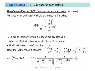
6. Max. Likelihood 6.1 Maximum likelihood method. Rao-Cramer-Frechet (RCF) bound of minimum variance (w/o proof) Variance of an estimator of single parameter is limited as: is called “efficient” when the bound exactly archived

E N D
6. Max. Likelihood 6.1 Maximum likelihood method • Rao-Cramer-Frechet (RCF) bound of minimum variance (w/o proof) • Variance of an estimator of single parameter is limited as: • is called “efficient” when the bound exactly archived • When an efficient estimator exists, it is a ML estimator • All ML estimators are efficient for n → ∞ • Example: exponential distribution : • as (b=0) : K. Desch – Statistical methods of data analysis SS10
6. Max. Likelihood 6.1 Maximum likelihood method Several parameters : RCF: “Fisher information matrix” V-1 ~ n and V ~ 1/n→ statistical errors decrease in proportion to (for efficient estimators) K. Desch – Statistical methods of data analysis SS10
6. Max. Likelihood 6.1 Maximum likelihood method Estimation of covariance matrix : Often difficult to be calculated Estimation through : For 1 parameter Determination of second derivative can be performed analytically or numerically K. Desch – Statistical methods of data analysis SS10
6. Max. Likelihood 6.1 Maximum likelihood method Graphical method for determination of variance : Expand logL(θ) in a Taylor series around the ML estimate : We know that : from RCF bound : (can be considered as definition of statistical error) For n → ∞ logL(θ) function becomes parabola ( vanish) When logL is not parabolic → asymmetrical errors central confidence interval K. Desch – Statistical methods of data analysis SS10
6. Max. Likelihood 6.1 Maximum likelihood method K. Desch – Statistical methods of data analysis SS10
6. Max. Likelihood 6.1 Maximum likelihood method Extended maximum likelihood (EML) Model makes predictions on normalization and form of distribution example: differential cross section (angular distribution) absolute normalization is Poisson distributed itself is a function of Extended likelihood function: 1. when then logarithm of EML: leads in general to smaller variance (smaller error) for as the estimator explores additional information from normalization K. Desch – Statistical methods of data analysis SS10
6. Max. Likelihood 6.1 Maximum likelihood method 2. independent parameter from ; one obtain the same estimators for Contributions to distribution f1,f2,f3 are known; relative contribution is not. p.d.f. : Parameters are not independent as ! One can define only m-1parameters by ML Symmetric – EML : K. Desch – Statistical methods of data analysis SS10
6. Max. Likelihood 6.1 Maximum likelihood method by defining (μi = expected number of events of type i) μi are no longer subject to constraints; each μjis Poisson mean Example : signal + background EML-fit of μs , μb→ can be negative when ? → bias → combination of many experiments has bias ! K. Desch – Statistical methods of data analysis SS10
6. Max. Likelihood 6.1 Maximum likelihood method Maximum likelihood with binned data For very large data samples log-likelihood function becomes difficult to compute → make a histogram for each measurement, yielding a central number of entries n = (n1,…,nN) in N bins. The expectation values of the number of entries are given by: where and are the bin limits The likelihood function is then : (does not depend on θ) Simpler to interpret when ?? K. Desch – Statistical methods of data analysis SS10
6. Max. Likelihood 6.1 Maximum likelihood method then : (when ni = 0 the [] should be substituted by when (→ method of least squares) For large ntot the binned ML method provides only slightly larger errors as unbinned ML Testing goodness-of-fit with maximum likelihood ML-method dos not directly suggest a method of testing “goodness-of-fit”. After successful fit the results must be checked for consitency K. Desch – Statistical methods of data analysis SS10
p.d.f. für Lmax P-Wert Lmax Observed Lmax 6. Max. Likelihood 6.1 Maximum likelihood method Possibilities: 1. MC study for Lmax: a) estimate from many MC experiments b) Histogram logLmax c) Compare with the observed Lmax from the real experiment d) Calculate “P-value” = probability for the observed parameter E[P]=50% (??) K. Desch – Statistical methods of data analysis SS10
6. Max. Likelihood 6.1 Maximum likelihood method -test divide sample into N bins and build : (ntot = free (Poisson), N-m d.o.f.) or : (ntot = fixed, N-m-1 d.o.f.) For large ntot the statistics given above follows exactly distribution or K. Desch – Statistical methods of data analysis SS10
6. Max. Likelihood 6.1 Maximum likelihood method Combining measurements with maximum likelihood Example : experiment with n measurements xi, p.d.f f(x;θ) second experiment with m measurements yi, p.d.f. f(y;θ) (same par. θ) → common likelihood function : or equivalently: → a common estimation of through max. of L(θ) Suppose two experiments based on a measurements of x and y give estimators and . One reports the estimated standard deviations and as the errors on and When and are independent, then K. Desch – Statistical methods of data analysis SS10