Download
1 / 19
200 likes | 325 Views
Assimilating Data into Earthquake Simulations. Michael Sachs, J.B. Rundle, D.L. Turcotte University of California, Davis Andrea Donnellan Jet Propulsion Laboratory. Data Assimilation, Model Steering, Model Tuning. Data = Model + Errors. Linearize. Matrix of Partial Derivatives.

E N D
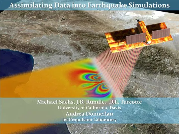
Assimilating Data into Earthquake Simulations Michael Sachs, J.B. Rundle, D.L. Turcotte University of California, Davis Andrea Donnellan Jet Propulsion Laboratory
Data Assimilation, Model Steering, Model Tuning Data = Model + Errors Linearize Matrix of Partial Derivatives
Applications Climate Models Numerical weather forecasting Global Ocean Data Assimilation Experiment http://www.usgodae.org/ DART (NCAR): Community DAta & Research Testbed) http://www.image.ucar.edu/DAReS/DART/ Land Data Assimilation Systems http://ldas.gsfc.nasa.gov/ Satellite Data Assimilation http://www.jcsda.noaa.gov/ Snow Data Assimilation System http://nsidc.org/data/g02158.html Orbit correction Financial markets and trading models Econometrics Engineering control systems
Kalman Filter From Wikipedia
Kalman Filter Solution
SCIDAC Tools for Computation, Data Assimilation, & Model Steering
Data Assimilation and Model Steering Using Automated Numerical Differentiators (e.g. ADIFOR -- FORTRAN) http://www.mcs.anl.gov/research/projects/adifor/
Data Assimilation and Model Steering Using Automated Numerical Differentiators (e.g. ADIC – ANSI C) http://www.mcs.anl.gov/research/projects/adic/
Other Standard Methods Linear Programming Simulated Annealing Genetic Algorithms & Evolutionary Programming Monte Carlo Search Simulations + Data Scoring
Data Assimilation via Scoring Method Compare Virtual California simulation data with historical seismic record Pick simulation times whose history is most similar to the historic data Use “future simulation times” to generate probabilities of future large events. J. Van Aalsburg et al., PEPI, 163, 149 (2007) J. Van Aalsburg et al., PAGEOPH, 167, 967 (2010)
Data Sets Virtual California 768 fault boundary elements in model 1.5 million events 200,000 years Paleoseismic Data 119 events 20 sites J. Van Aalsburg et al., PEPI, 163, 149 (2007) J. Van Aalsburg et al., PAGEOPH, 167, 967 (2010)
1.0 Score Area Under Gaussian Curve = 1 0.0 Paleo Date Std. Dev. Simulation Event Assimilation (Scoring) Algorithm Associate VC segments with paleo sites single-site pair (nearest-neighbor) specified radius (long-range neighborhood) Select scoring method and generate scoring functions “Score” the simulation data We use a “unit area Gaussian” scoring function
1.0 Score Area Under Gaussian Curve = 1 0.0 Paleo Date Std. Dev. Simulation Event Gaussian Scoring Score Simulation Time (years) Gaussian Scoring Function
Time-space plot of the dynamics: Coulomb failure stress (colors), earthquakes (horizontal lines) for all segments in the model. Forecast Window Log [ 1-CFF(x,t) ] Color Cycle 2000 Years of Elapsed Time Evaluation Window Time (Yr) Space (Distance, km) Optimal Forecast Interval Creeping Garlock NSAF SSAF Stress Dynamics and the Optimization of Numerical Forecasts using “Data-Scoring” Which epochs of simulation data are most like the observed data? Using only the intervals following these epochs will allow us to optimize forecast statistics. Data Score Plots from Weldon (2005) Time
High Scoring Event Low Scoring Event High and Low Scoring Events: Virtual California - Paleoseismology
Spatial & Temporal PDFs Determine magnitude threshold (magnitude > m) Use m = 7.0 for temporal pdf Use m = 6.5 and m = 7.0 for spatial pdf Set a decision threshold (approx. 1% of simulation data) Temporal: Starting at these “high scoring” years compute the time until the next large event having m > 7.0 Spatial: For each “high scoring” year, determine boundary elements that participate in the next m > 6.5 and m > 7.0 events
Temporal Waiting Time Statistics: Starting at these “high scoring” years compute the time until the next large event having m > 7.0 Then find the most likely locations for these events Waiting Time Distribution 0 5 10 15 20 25 30 Time (years)
Spatial Probability Density Functions: For each “high scoring” year, determine the boundary elements that tend to participate in the next m > 6.5 and m > 7.0 events Spatial Probability Density for next event m > 6.5 Peak value = 0.253 Spatial Probability Density for next event m > 7.0 Peak value = 0.214
Results Temporal: 50% probability that the next large event with m > 7.0 will occur within ~ 8 years Probability distribution is nearly Poisson due to incoherent stacking of data from many fault elements Spatial: Next event having m > 6.5 most likely to occur on Calaveras fault Next event having m > 7.0 most likely to occur on either Carrizo plain segment of San Andreas fault, northern San Andreas, or Garlock faults