Download
1 / 61
610 likes | 800 Views
New Surprises from Self-Reducibility. CiE 2010, Ponta Delgada, Azores. Why a “Fantastic Voyage”?. It’s apt. It’s a bad pun on “self-reduction”. It is contemporary with the birth of self-reducibility. 40 Years of Self-Reducibility.

E N D
New Surprises from Self-Reducibility CiE 2010, Ponta Delgada, Azores
Why a “Fantastic Voyage”? • It’s apt. • It’s a bad pun on “self-reduction”. • It is contemporary with the birth of self-reducibility.
40 Years of Self-Reducibility • Boris A. Trakhtenbrot, On Autoreducibility, Dokl. Akad. Nauk. SSSR 11, 1970.
Self-Reducibility • A set B is said to be “self-reducible” if B≤rB
Self-Reducibility • A set B is said to be “self-reducible” if B≤rB via a reduction that, on input x, does not ask about whether x is in B. • Very well-studied notion. • For example, φ is in SAT if and only if (φ0 is in SAT) or(φ1 is in SAT).
Self-Reducibility • A set B is said to be “self-reducible” if B≤rB via a reduction that, on input x, does not ask about whether x is in B. • Very well-studied notion. • In fact, this is such a simple notion, the really surprising thing is that, for four decades, slight variations on this theme have yielded surprising and powerful insights. • We will not survey all 40 years of work on this topic! (See [Selke].)
Plan for Today • Give a brief review of some (historical) settings where self-reducibility has been useful in complexity theory. • Present a few recent examples of work at the intersection of complexity theory and computability theory, where self-reducibility plays a central role. • But first, let’s recall some of the grand challenges in complexity theory that motivate these investigations.
What Crypto Needs from Complexity • Factoring (or some other suitable trap-door function) is hard for some fixed input size (corresponding to the size of a public key). • That is: we need to talk about hardness of finite functions. • Complexity theory can do this: • Theorem: Any circuit that takes as input a logical formula (in WS1S) of length 616 and produces as output a correct answer, saying if the formula is valid or not, has at least 10123 gates. (Stockmeyer, 1974)
Circuits vs Turing Machines • 2 Basic models of computation • Programs (one program – works for every input length) • Circuits (different circuit for each input length) • One crucial difference: circuit lower bounds can be used to prove intractability results for fixed input sizes. • Program run-time lower bounds can’t.
An example: the Game of Checkers • Computing strategies for Checkers requires exponential time. • More precisely, given an n-by-n Checkers board with checkers on it, no program can compute an optimal next move in fewer than c2n – d steps, for some constants c and d. • n-by-n Checkers is complete for EXP.
An example: the Game of Checkers • Computing strategies for Checkers requires exponential time. • More precisely, given an n-by-n Checkers board with checkers on it, no program can compute an optimal next move in fewer than c2n – d steps, for some constants c and d. • Thus any program solving this problem must run very slowly on large inputs. This is the essence of asymptotic analysis.
An example: the Game of Checkers • Computing strategies for Checkers requires exponential time. • More precisely, given an n-by-n Checkers board with checkers on it, no program can compute an optimal next move in fewer than c2n – d steps, for some constants c and d. • but…Conceivably, there is a hand-held device that computes optimal moves, even for Checker boards of size 1000-by-1000! • …because we don’t know if EXP is in P/poly (the class of problems with small circuits).
Two Fundamental Questions: SAT є P SAT є P/poly [Karp-Lipton, 1980] coNPNP = NPNP
Two Fundamental Questions: SAT є P SAT є P/poly [Karp-Lipton, 1980] coNPNP = NPNP Guess a circuit, and use the NP oracle to see if it computes SAT.
Autoreducibility of Complete Sets • Here are a few longstanding open questions in complexity theory: • EXP = NP • EXP = PH (= NP U NPNP U NPNPNP …) • PSPACE = NP • PSPACE = PH (= NP U NPNP U NPNPNP …) • [Buhrman, Fortnow, van Melkebeek, Torenvliet] showed that resolving some innocent-sounding questions about auto-reducibility would solve these questions!
Autoreducibility of Complete Sets • [BFvMT]: All ≤P-Complete sets for EXP are autoreducible. • There is an oracle A, relative to which not all ≤P-Complete sets for EXP are autoreducible. • Thus the proof of the preceding theorem does not “relativize”. (That’s a good thing!) • Not all ≤P-Complete sets for EEXPSPACE (doubly-exponential space) are autoreducible. • How about classes between EXP and EEXPSPACE? (E.g., EXPSPACE & EEXP.)
Autoreducibility of Complete Sets • Are all ≤P-Complete sets for EEXP autoreducible? • If YES, then PH ≠ EXP. • If NO, then P ≠ PSPACE. • Are all ≤P-Complete sets for EXPSPACE autoreducible? • Usually questions about “big” classes like EXPSPACE and EEXP are not too hard to answer. Diagonalization techniques work there, that don’t work for “smaller” classes.
Autoreducibility of Complete Sets • Are all ≤P-Complete sets for EEXP autoreducible? • If YES, then PH ≠ EXP. • If NO, then P ≠ PSPACE. • Are all ≤P-Complete sets for EXPSPACE autoreducible? • If YES then PH ≠ PSPACE.
Autoreducibility of Complete Sets • Are all ≤P-Complete sets for EEXP autoreducible? • If YES, then PH ≠ EXP. • If NO, then P ≠ PSPACE & NL ≠ NP. • Are all ≤P-Complete sets for EXPSPACE autoreducible? • If YES then PH ≠ PSPACE. • If NO, then NL ≠ NP.
Big Complexity Classes • NP • P • . • . • NC • NL (Nondeterministic Logspace) • L (Deterministic Logspace)
Objects of Interest:Small Complexity Classes • TC0O(1)-Depth Circuits of MAJ gates • AC0 [6] • NC1 Log-Depth Circuits • AC0 can’t compute Mod 2 [FSS,A] • AC0 O(1)-Depth Circuits of AND/OR gates
Objects of Interest:Small Complexity Classes • TC0O(1)-Depth Circuits of MAJ gates • AC0 [6] • NC1 Log-Depth Circuits • AC0 can’t compute Mod 2 [FSS,A] • AC0 O(1)-Depth Circuits of AND/OR gates
Objects of Interest:Small Complexity Classes • TC0O(1)-Depth Circuits of MAJ gates • NC1 Log-Depth Circuits • AC0 [2]can’t compute Mod 3 [R,S] • AC0 [2] • AC0 O(1)-Depth Circuits of AND/OR gates
Objects of Interest:Small Complexity Classes • NC1 Log-Depth Circuits • TC0O(1)-Depth Circuits of MAJ gates • AC0 [6] • AC0 [2] • AC0 O(1)-Depth Circuits of AND/OR gates
Objects of Interest:Small Complexity Classes • NC1 poly-size formulae • TC0O(1)-Depth Circuits of MAJ gates • AC0 [6] • AC0 [2] • AC0 O(1)-Depth Circuits of AND/OR gates
Complete Problems • NP has complete sets (under polynomial time reducibility ≤P) • These small classes have complete sets, too (under ≤AC°) • Amazingly, even with restricted reductions, the classes of complete sets for “big” complexity classes (EXP, NP, …) are essentially unchanged.
Reductions • A ≤AC°B means that there is a constant-depth circuit computing A that has the usual AND and OR gates, and also has ‘oracle gates’ for B. B
Complete Problems • NC1 • TC0 • AC0 [6] • AC0 [2] • AC0 • sorting, multiplication, division • [Naor,Reingold] Pseudorandom Generator
Complete Problems • NC1 • TC0 • AC0 [6] • AC0 [2] • AC0 • BFE: Balanced Boolean Formula Evaluation (AND,OR,XOR) • Word problem over S5
The Word Problem Over S5 • A regular set complete for NC1 =
Complexity Classes are not Invented – They’re Discovered • NP (SAT, Clique, TSP,…) • P (Linear Programming, CVP, …) • NL (Connectivity, Shortest Paths, 2SAT, …) • L (Undirected Connectivity, Acyclicity, …) • NC1 (BFE, Regular Sets) • TC0 (Sorting, Multiplication, Division) We’re interested in NC1 (for instance) not because we want to build formulae for these functions…
Complexity Classes are not Invented – They’re Discovered • NP (SAT, Clique, TSP,…) • P (Linear Programming, CVP, …) • NL (Connectivity, Shortest Paths, 2SAT, …) • L (Undirected Connectivity, Acyclicity, …) • NC1 (BFE, Regular Sets) • TC0 (Sorting, Multiplication, Division) … but because we want to know if the blocks of this partition are distinct.
Complexity Classes are not Invented – They’re Discovered • NP (SAT, Clique, TSP,…) • P (Linear Programming, CVP, …) • NL (Connectivity, Shortest Paths, 2SAT, …) • L (Undirected Connectivity, Acyclicity, …) • NC1 (BFE, Regular Sets) • TC0 (Sorting, Multiplication, Division) These classes are real. They’re important.
Other Longstanding Open Problems • Is P = NP? • Is AC0[6] = NP? • Is depth 3 AC0[6] = NP? We’ll focus on questions such as: Is BFE in TC0? Is BFE in AC0[6]?
How Close Are We to Proving Circuit Lower Bounds? • Conventional Wisdom: Not Close At All! • No new superpolynomial size lower bounds in over two decades. • Razborov and Rudich: Any “natural” argument proving a lower bound against a circuit class C yields a proof that C can’t compute a pseudorandom function generator. • Since the [Naor, Reingold] generator is computable in TC0, this is bad news.
More Modest Goals • Problems requiring formulae of size n3 [Håstad] • Problems requiring branching programs of size nearly n loglog n [Beame, Saks, Sun, Vee] • Problems requiring depth d TC0 circuits of size n1+c [Impagliazzo, Paturi, Saks] • Time-Space Tradeoffs [Fortnow, Lipton, Van Melkebeek, Viglas] • There is little feeling that these results bring us any closer to separating complexity classes.
How Close Are We to Proving Circuit Lower Bounds? • How close are the following two statements? • TC0 Circuits for BFE must be of size n1+Ω(1) • For some c>0, TC0 Circuits for BFE must be of size n1+c.
How Close Are We to Proving Circuit Lower Bounds? • How close are the following two statements? • TC0 Circuits for BFE must be of size n1+Ω(1) • For some c>0, TC0 Circuits for BFE must be of size n1+c This is known [IPS’97] This implies TC0≠ NC1 [A, Koucky]
Self-Reducibility • [Goldwasser et al]: Many of the important problems in (or near) NC1 have a special self-reducibility property:
Self-Reducibility • [Goldwasser et al]: Many of the important problems in (or near) NC1 have a special self-reducibility property: Instances of length n are AC0-Turing reducible to instances of length n½ via reductions of linear size. • Examples: • BFE • the word problem over S5 • MAJORITY
Self Reducibility • BFE A subformula near the root Subformulae near inputs
Self Reducibility • S5
Self Reducibility • The self-reduction of S5, on inputs of size n, uses (n½ + 1) oracle gates of size n½. • Thus if S5 has TC0 circuits of size nk, it also has circuits of size (n½ + 1)nk/2= O(n(k+1)/2). • Similar arguments hold for other classes (such as AC0[6] and NC1). • More complicated self-reductions can be presented for MAJORITY and other problems.
A Corollary • If BFE has TC0 or AC0[6] circuits, then it has such circuits of nearly linear size. • If S5 has TC0 or AC0[6] circuits, then it has such circuits of nearly linear size. • If MAJ has AC0[6] circuits, then it has such circuits of nearly linear size. (Etc.) • Thus, e.g., to separate NC1 from TC0, it suffices to show that BFE requires TC0 circuits of size n1.0000001.
Prospects for Progress • The [Razborov & Rudich] framework of natural proofs assumes that a “natural” proof of a lower bound will make use of a combinatorial property that (among other things) is shared by a large fraction of the functions on n bits. • In contrast, we are making use of a self-reducibility property that allows us to boost a n1+ε lower bound to a superpolynomial lower bound. This self-reducibility property holds for only a vanishingly small fraction of all functions.
Prospects for Progress • The [Razborov & Rudich] framework of natural proofs assumes that a “natural” proof of a lower bound will make use of a combinatorial property that (among other things) is shared by a large fraction of the functions on n bits. • Thus, it’s conceivable that a “natural” proof can be given of a modest lower bound of the form: BFE requires TC0 circuits of size n1.0000001. This would yield an “unnatural” proof separating NC1 from TC0.
Recall… • If BFE has TC0 or AC0[6] circuits, then it has such circuits of nearly linear size. • If S5 has TC0 or AC0[6] circuits, then it has such circuits of nearly linear size. • If MAJ has AC0[6] circuits, then it has such circuits of nearly linear size. (Etc.) • How widespread is this phenomenon? Is it true for SAT? (I.e., if SAT is in TC0, does it have TC0 circuits of size n1.0000001?)