Query Processing: From High Level Queries to Optimized Plans
1.44k likes | 1.45k Views
Learn how the query processor transforms user queries into efficient query plans by making decisions on algebraic operators, data passing, and algorithm selection. Explore the journey of a query from parsing to obtaining the optimal plan.

Query Processing: From High Level Queries to Optimized Plans
E N D
Presentation Transcript
Query Processing • The query processor turns user queries and data modification commands into a query plan - a sequence of operations (or algorithm) on the database • from high level queries to low level commands • Decisions taken by the query processor • Which of the algebraically equivalent forms of a query will lead to the most efficient algorithm? • For each algebraic operator what algorithm should we use to run the operator? • How should the operators pass data from one to the other? (eg, main memory buffers, disk buffers)
Example Select B,D From R,S Where R.A = “c” S.E = 2 R.C=S.C
Answer B D 2 x R A B C S C D E a 1 10 10 x 2 b 1 20 20 y 2 c 2 10 30 z 2 d 2 35 40 x 1 e 3 45 50 y 3
How do we execute query eventually? - Scan relations - Do Cartesian product - Select tuples - Do projection One idea
Bingo! Got one... RxS R.A R.B R.C S.C S.D S.E a 1 10 10 x 2 a 1 10 20 y 2 . . C 2 10 10 x 2 . .
Relational Algebra - can be enhanced to describe plans... OR:B,D [sR.A=“c” S.E=2 R.C = S.C (R X S )] FLY SCAN SCAN FLY • Scan R • For each tuple r of R scan S • For each (r,s), where s in S • select and project on the fly Ex: Plan I B,D sR.A=“c” S.E=2 R.C=S.C X R S FLY FLY SCAN SCAN
“FLY” and “SCAN” are the defaults Ex: Plan I B,D sR.A=“c” S.E=2 R.C=S.C X R S
Another idea: B,D sR.A = “c”sS.E = 2 R S Plan II HASH natural join Scan R and S, perform on the fly selections, do hash join, project
R S A B C s (R) s(S) C D E a 1 10 A B C C D E 10 x 2 b 1 20 c 2 10 10 x 2 20 y 2 c 2 10 20 y 2 30 z 2 d 2 35 30 z 2 40 x 1 e 3 45 50 y 3
Plan III Use R.A and S.C Indexes (1) Use R.A index to select R tuples with R.A = “c” (2) For each R.C value found, use S.C index to find matching join tuples (3) Eliminate join tuples S.E 2 (4) Project B,D attributes
=“c” <c,2,10> <10,x,2> check=2? output: <2,x> next tuple: <c,7,15> R S A B C C D E a 1 10 10 x 2 b 1 20 20 y 2 c 2 10 30 z 2 d 2 35 40 x 1 e 3 45 50 y 3 A C I1 I2
Algebraic Form of Plan p R.B, S.D s Right Index Join S.E=2 RI INDEX s R.a=“c” S R
From Query To Optimal Plan • Complex process • Algebra-based logical and physical plans • Transformations • Evaluation of multiple alternatives
Issues in Query Processing and Optimization • Generate Plans • employ efficient execution primitives for computing relational algebra operations • systematically transform expressions to achieve more efficient combinations of operators • Estimate Cost of Generated Plans • Statistics • “Smart” Search of the Space of Possible Plans • always do the “good” transformations (relational algebra optimization) • prune the space (e.g., System R) • Often the above steps are mixed
SQL query parse answer parse tree execute convert statistics Pi logical query plan pick best Generate/Transform lqp’s {(P1,C1),(P2,C2)...} “improved” l.q.p(s) estimate costs estimate result sizes l.q.p. +sizes Generate/Transform pqp’s generate physical plans {P1,P2,…..} Scope of responsibility of each module may is fuzzy
Example: The Journey of a Query Initial logical query plan SELECT Theater FROM Movie M, Schedule S WHERE M.Title = S.Title AND M.Actor=“Winger” p Theater Parse/ Convert s M.Title=S.Title AND M.Actor=“Winger” x Movie Schedule Logical Plan Generator applies Algebraic Rewriting And yet another logical query plan p Theater Another logical query plan p s Theater M.Actor=“Winger” Logical Plan Generator s M.Title=S.Title M.Actor=“Winger” JOIN s M.Title=S.Title Movie Schedule x Next Page Movie Schedule
The Journey of a Query cont’d: Summary of Logical Plan Generator p p 4th logical query plan Theater Theater s S.Title=M.Title M.Actor=“Winger” Logical Plan Generator M.Title=S.Title s M.Actor=“Winger” Schedule Movie Movie Schedule • 4 logical query plans created • algebraic rewritings were used for producing the candidate logical query plans plans • the last one is the winner (at least, cannot be a big loser) • in general, multiple logical plans may “win” eventually if cond refers only on S s cond s x cond R R S S
The Journey of a Query Continues at the Physical Plan Generator p Theater index on Actor, tables Schedule sorted on Title, Physical Plan Generator S.Title=M.Title p Theater SORT-MERGE s S.Title=M.Title M.Actor=“Winger” Schedule Movie INDEX s • M.Actor=“Winger” Physical Plan Generators chooses execution primitives and data passing Schedule Movie index on Actor and Title, unsorted tables, tables>>memory Physical Plan 2 p Theater LEFT INDEX S.Title=M.Title More than one plans may be generated by choosing different primitives Physical Plan 1 INDEX s • Actor=“Winger” Schedule Movie
Example: Nested SQL query SELECT title FROM StarsIn WHERE starName IN ( SELECT name FROM MovieStar WHERE birthdate LIKE ‘%1960’ ); (Find the movies with stars born in 1960)
Example: Parse Tree <Query> <SFW> SELECT <SelList> FROM <FromList> WHERE <Condition> <Attribute> <RelName> <Tuple> IN <Query> title StarsIn <Attribute> ( <Query> ) starName <SFW> SELECT <SelList> FROM <FromList> WHERE <Condition> <Attribute> <RelName> <Attribute> LIKE <Pattern> name MovieStar birthDate ‘%1960’
Example: Generating Relational Algebra title StarsIn <condition> <tuple> IN name <attribute> birthdate LIKE ‘%1960’ starName MovieStar An expression using a two-argument , midway between a parse tree and relational algebra
Example: Logical Query Plan (Relational Algebra) title starName=name StarsIn name birthdate LIKE ‘%1960’ MovieStar May consider “IN” elimination as a rewriting in the logical plan generator or may consider it a task of the converter
Example: Improved Logical Query Plan title Question: Push project to StarsIn? starName=name StarsIn name birthdate LIKE ‘%1960’ MovieStar
Example: Result sizes are important for selecting physical plans Need expected size StarsIn MovieStar P s
Example: One Physical Plan Additional parameters: memory size, result sizes... title starName=name name INDEX s SCAN • birthdate LIKE ‘%1960’ StarsIn MovieStar
Topics • Bag Algebra and other extensions • name & value conversions, functions, aggregation
Algebraic Operators: A Bag version • Union of R and S: a tuple t is in the result as many times as the sum of the number of times it is in R plus the times it is in S • Intersection of R and S: a tuple t is in the result the minimum of the number of times it is in R and S • Difference of R and S: a tuple t is in the result the number of times it is in R minus the number of times it is in S • (R)converts the bag R into a set • SQL’s R UNION S is really (R S) • Example: Let R={A,B,B} and S={C,A,B,C}.Describe the union, intersection and difference...
Extended Projection • We extend the relational project pAas follows: • The attribute list may include xy in the list A to indicate that the attribute x is renamed to y • Arithmetic or string operators on attributes are allowed. For example, • a+bx means that the sum of a and b is renamed into x. • c||dy concatenates the result of c and d into a new attribute named y • The result is computed by considering each tuple in turnand constructing a new tuple by picking the attributes names in A and applying renamings and arithmetic and string operators • Example:
An Alternative Approach to Arithmetic and Other 1-1 Computations • Special purpose operators that for every input tuple they produce one output tuple • MULTA,BCR: for each tuple of R, multiply attribute A with attribute B and put the result in a new attribute named C. • PLUSA,BCR • CONCATA,BCR • Exercise: Write the above operators using extended projection. Assume the schema of R is R(A,B,D,E).
Product and Joins • Product of R and S (RS): • If an attribute named a is found in both schemas then rename one column into R.a and the other into S.a • If a tuple r is found n times in R and a tuple s is found m times in S then the product contains nm instances of the tuple rs • Joins • Natural JoinR S = pA sC(RS) where • C is a condition that equates all common attributes • A is the concatenated list of attributes of R and S with no duplicates • you may view tha above as a rewriting rule • Theta Join • arbitrary condition involving multiple attributes
Grouping and Aggregation • Operators that combine the GROUP-BY clause with the aggregation operator (AVG,SUM,MIN,MAX,…) • SUMGroupbyList;GroupedAttributeResultAttribute R corresponds to SELECT GroupbyList, SUM(GroupedAttribute) AS ResultAttribute FROM R GROUP BY GroupbyList • Similar for AVG,MIN,MAX,COUNT… • Note that (R) could be seen as a special case of grouping and aggregation • Example
Relational algebra optimization • Transformation rules (preserve equivalence) • What are good transformations?
Algebraic Rewritings: Commutativity and Associativity Commutativity Associativity Cartesian Product T R R S S R R S S T Natural Join T R R S S R R S S T Question 1: Do the above hold for both sets and bags? Question 2: Do commutativity and associativity hold for arbitrary Theta Joins?
Algebraic Rewritings: Commutativity and Associativity (2) Commutativity Associativity Union T R R S S R R S S T Intersection T R R S S R R S S T Question 1: Do the above hold for both sets and bags? Question 2: Is difference commutative and associative?
Algebraic Rewritings for Selection: Decomposition of Logical Connectives s cond1 s cond2 R s s cond1 AND cond2 cond2 R s cond1 R Does it apply to bags? s cond1 OR cond2 s s cond1 cond2 R R
Algebraic Rewritings for Selection: Decomposition of Negation Complete Question s cond1 AND NOT cond2 R s NOT cond2 R s cond1 OR NOT cond2 R
Pushing the Selection Thru Binary Operators: Union and Difference s cond Union s s cond cond R S R S - Difference s s s cond cond cond - R S - R S s cond R S Exercise: Do the rule for intersection
Pushing Selection thru Cartesian Product and Join s The right direction requires that cond refers to S attributes only cond s cond R R S S s The right direction requires that cond refers to S attributes only cond s cond R R S S The right direction requires that all the attributes used by cond appear in both R and S s cond s cond S R Exercise: Do the rule for theta join
Rules:p,s combined pxz px Let x = subset of R attributes z = attributes in predicate P (subset of R attributes) px[sp (R) ] = {sp [ px (R) ]}
Pushing Simple Projections Thru Binary Operators A projection is simple if it only consists of an attribute list A Union A A R S R S Question 1: Does the above hold for both bags and sets? Question 2: Can projection be pushed below intersection and difference? Answer for both bags and sets.
Pushing Simple Projections Thru Binary Operators: Join and Cartesian Product Where B is the list of R attributes that appear in A. Similar for C. A A R S B C R S Question: What is B and C ? A A R S B C R S Exercise: Write the rewriting rule that pushes projection below theta join.
Projection Decomposition p X p p X XY R R
Some Rewriting Rules Related to Aggregation: SUM • scondSUMGroupbyList;GroupedAttributeResultAttributeR SUMGroupbyList;GroupedAttributeResultAttribute scond R, if cond involves only the GroupbyList • SUMGL;GARA(RS) PLUS RA1, RA2:RA ((SUMGL;GARA11 R) (SUMGL;GARA2 S))) • SUM GL2;RA1RA2 SUM GL1;GARA1R SUMGL2:GARA2R • Question: does the above hold for both bags and sets?
Derived Rules:s + combined More Rules can be Derived: spq (R S) = spqm (R S) = spvq (R S) = p only at R, q only at S, m at both R and S
--> Derivation for first one: spq (R S) = sp [sq (R S) ] = sp[ R sq (S) ] = [sp (R)] [sq (S)]
Which are always “good” transformations? sp1p2 (R) sp1 [sp2 (R)] sp (R S) [sp (R)] S R S S R px [sp(R)] px {sp [pxz(R)]}
In textbook: more transformations • Eliminate common sub-expressions • Other operations: duplicate elimination
Bottom line: • No transformation is always good at the l.q.p level • Usually good: • early selections • elimination of cartesian products • elimination of redundant subexpressions • Many transformations lead to “promising” plans • Commuting/rearranging joins • In practice too “combinatorially explosive” to be handled as rewriting of l.q.p.
Arranging the Join Order: the Wong-Youssefi algorithm (INGRES) Sample TPC-H Schema Nation(NationKey, NName) Customer(CustKey, CName, NationKey) Order(OrderKey, CustKey, Status) Lineitem(OrderKey, PartKey, Quantity) Product(SuppKey, PartKey, PName) Supplier(SuppKey, SName) Find the names of suppliers that sell a product that appears in a line item of an order made by a customer who is in Canada SELECT SName FROM Nation, Customer, Order, LineItem, Product, Supplier WHERE Nation.NationKey = Cuctomer.NationKey AND Customer.CustKey = Order.CustKey AND Order.OrderKey=LineItem.OrderKey AND LineItem.PartKey= Product.Partkey AND Product.Suppkey = Supplier.SuppKey AND NName = “Canada”

