Download
1 / 42
420 likes | 440 Views
This text covers data sources, role of hypothesis, exploring distributions, and testing and evaluating results in data analytics.

E N D
Data and Information Resources, Role of Hypothesis, Exploration and Distributions Peter Fox Data Analytics – ITWS-4963/ITWS-6965 Week 2a, February 2, 2016, LALLY 102
Contents • Data sources • Cyber • Human • “Munging” • Exploring • Distributions… • Summaries • Visualization • Testing and evaluating the results (beginning)
Data Prepared for Analysis = Munging • Missing values, null values, etc. • E.g. in the EPI_data – they use “--” • Most data applications provide built ins for these higher-order functions – in R “NA” is used and functions such as is.na(var), etc. provide powerful filtering options (we’ll cover these on Friday) • Of course, different variables often are missing “different” values • In R – higher-order functions such as: Reduce, Filter, Map, Find, Position and Negate will become your enemies and then your friends: http://www.johnmyleswhite.com/notebook/2010/09/23/higher-order-functions-in-r/
Getting started – summarize data • Summary statistic • Ranges, “hinges” • Tukey’s five numbers • Look for a distribution match • Tests…for… • Normality – shapiro-wilks – returns a statistic (W!) and a p-value – what is the null hypothesis here? > shapiro.test(EPI_data$EPI) Shapiro-Wilk normality test data: EPI_data$EPI W = 0.9866, p-value = 0.1188
Accept or Reject? • Reject the null hypothesis if the p-value is less than the level of significance. • You will fail to reject the null hypothesis if the p-value is greater than or equal to the level of significance. • Typical significance 0.05 (!)
Another variable in EPI > shapiro.test(EPI_data$DALY) Shapiro-Wilk normality test data: EPI_data$DALY W = 0.9365, p-value = 1.891e-07 Accept or reject?
Distribution tests • Binomial, …. most distributions have tests • Wilcoxon (Mann-Whitney) • Comparing populations – versus to a distribution • Kolmogorov-Smirnov (KS) • … • It got out of control when people realized they can name the test after themselves, v. someone else…
Getting started – look at the data • Visually • What is the improvement in the understanding of the data as compared to the situation without visualization? • Which visualization techniques are suitable for one's data? • Scatter plot diagrams • Box plots (min, 1st quartile, median, 3rd quartile, max) • Stem and leaf plots • Frequency plots • Group Frequency Distributions plot • Cumulative Frequency plots • Distribution plots
Why visualization? • Reducing amount of data, quantization • Patterns • Features • Events • Trends • Irregularities • Leading to presentation of data, i.e. information products • Exit points for analysis
Exploring the distribution > summary(EPI) # stats Min. 1st Qu. Median Mean 3rd Qu. Max. NA's 32.10 48.60 59.20 58.37 67.60 93.50 68 > boxplot(EPI) > fivenum(EPI,na.rm=TRUE) [1] 32.1 48.6 59.2 67.6 93.5 Tukey: min, lower hinge, median, upper hinge, max
Stem and leaf plot > stem(EPI) # like-a histogram The decimal point is 1 digit(s) to the right of the | - but the scale of the stem is 10… watch carefully.. 3 | 234 3 | 66889 4 | 00011112222223344444 4 | 5555677788888999 5 | 0000111111111244444 5 | 55666677778888999999 6 | 000001111111222333344444 6 | 5555666666677778888889999999 7 | 000111233333334 7 | 5567888 8 | 11 8 | 669 9 | 4
Grouped Frequency Distribution aka binning > hist(EPI) #defaults
Distributions • Shape • Character • Parameter(s) • Which one fits?
> hist(EPI, seq(30., 95., 1.0), prob=TRUE) • > lines (density(EPI,na.rm=TRUE,bw=1.)) • > rug(EPI) • or • > lines (density(EPI,na.rm=TRUE,bw=“SJ”))
> hist(EPI, seq(30., 95., 1.0), prob=TRUE) • > lines (density(EPI,na.rm=TRUE,bw=“SJ”))
> xn<-seq(30,95,1) > qn<-dnorm(xn,mean=63, sd=5,log=FALSE) > lines(xn,qn) > lines(xn,.4*qn) > ln<-dnorm(xn,mean=44, sd=5,log=FALSE) > lines(xn,.26*ln)
Exploring the distribution > summary(DALY) # stats Min. 1st Qu. Median Mean 3rd Qu. Max. NA's 0.00 37.19 60.35 53.94 71.97 91.50 39 > fivenum(DALY,na.rm=TRUE) [1] 0.000 36.955 60.350 72.320 91.500 EPI DALY
Stem and leaf plot > stem(DALY) # The decimal point is 1 digit(s) to the right of the | 0 | 0000111244 0 | 567899 1 | 0234 1 | 56688 2 | 000123 2 | 5667889 3 | 00001134 3 | 5678899 4 | 00011223444 4 | 555799 5 | 12223344 5 | 556667788999999 6 | 0000011111222233334444 6 | 6666666677788889999 7 | 00000000223333444 7 | 66888999 8 | 1113333333 8 | 555557777777777799999 9 | 22
Beyond histograms • Cumulative distribution function: probability that a real-valued random variable X with a given probability distribution will be found at a value less than or equal to x. > plot(ecdf(EPI), do.points=FALSE, verticals=TRUE)
Beyond histograms • Quantile ~ inverse cumulative density function – points taken at regular intervals from the CDF, e.g. 2-quantiles=median, 4-quantiles=quartiles • Quantile-Quantile (versus default=normal dist.) > par(pty="s") > qqnorm(EPI); qqline(EPI)
Beyond histograms • Simulated data from t-distribution (random): > x <- rt(250, df = 5) > qqnorm(x); qqline(x)
Beyond histograms • Q-Q plot against the generating distribution: x<-seq(30,95,1) > qqplot(qt(ppoints(250), df = 5), x, xlab = "Q-Q plot for t dsn") > qqline(x)
But if you are not sure it is normal > wilcox.test(EPI,DALY) Wilcoxon rank sum test with continuity correction data: EPI and DALY W = 15970, p-value = 0.7386 alternative hypothesis: true location shift is not equal to 0
Comparing the CDFs > plot(ecdf(EPI), do.points=FALSE, verticals=TRUE) > plot(ecdf(DALY), do.points=FALSE, verticals=TRUE, add=TRUE)
More munging • Bad values, outliers, corrupted entries, thresholds … • Noise reduction – low-pass filtering, binning • Modal filtering • REMEMBER: when you munge you MUST record what you did (and why) and save copies of pre- and post- operations…
Populations within populations • In the EPI example: • Geographic regions (GEO_subregion) • EPI_regions • Eco-regions (EDC v. LEDC – know what that is?) • Primary industry(ies) • Climate region • What would you do to start exploring?
Or, a twist – n=1 but many attributes? The item of interest in relation to its attributes
Summary: explore • Going from preliminary to initial analysis… • Determining if there is one or more common distributions involved – i.e. parametric statistics (assumes or asserts a probability distribution) • Fitting that distribution -> provides a model! • Or NOT • A hybrid or • Non-parametric (statistics) approaches are needed – more on this to come
Goodness of fit • And, we cannot take the models at face value, we must assess how fit they may be: • Chi-Square • One-sided and two-sided Kolmogorov-Smirnov tests • Lilliefors tests • Ansari-Bradley tests • Jarque-Bera tests • Just a preview…
Summary • Cyber and Human data; quality, uncertainty and bias – you will often spend a lot of time with the data • Distributions – the common and not-so common ones and how cyber and human data can have distinct distributions • How simple statistical distributions can mislead us • Populations and samples and how inferential statistics will lead us to model choices (no we have not actually done that yet in detail) • Munging toward exploratory analysis • Toward models!
How are the software installs going? • R • Data exercises? • You can try some of the examples from today on the EPI dataset • More on Friday… and other datasets.