Download
1 / 20
200 likes | 207 Views
SPATS – a South Pole Acoustic Test Setup. 1 st International ARENA Workshop Zeuthen May 2005. Overview. Motivation Experimental Targets Absorption and Scattering Speed of sound and refraction Background noise and transient events Setup In-ice components Data acquisition

E N D
SPATS –a South Pole Acoustic Test Setup 1st International ARENA Workshop Zeuthen May 2005
Overview • Motivation • Experimental Targets • Absorption and Scattering • Speed of sound and refraction • Background noise and transient events • Setup • In-ice components • Data acquisition • Networking and synchronisation • Organization • Collaboration • Project schedule • Summary
Motivation • Hybrid Optical-Radio-Acoustic array a most powerful neutrino observatory • Relevant acoustic properties of south polar ice are unknown Dedicated setup to determine acoustic properties
Experimental Targets • Aim: measure all relevant parameters needed for an acoustic detector proposal • Absorption length sensor density and possible detector volume • Velocity of sound and refraction signal shape and vertical sensor spacing • Ambient noise energy threshold • Transient background events signal-to-noise event ratio
Scattering B. Price, University Berkeley • Dominant process: • Rayleigh scattering at crystal boundaries crystal size frequency • λs ∝ a3 × f4 • Theoretical values • λs (10 kHz) ≈ 800 km • λs (100 kHz) ≈ 0.2 km • can (probably) be neglected
Absorption B. Price, University Berkeley • Dominant process: • molecular reorientation energy loss in relaxation • temperature dependant • crystal size dependant • Theoretical calculation: λa (-51℃) ≈ 7.1 km largest in upper ice layers J. Vandenbroucke, University Berkeley
Speed of sound • Speedof sound • weak temperature dependance • strong density dependance • very distinct kink profile refraction of surface noise • Measurement: • In same layer • Inter-layer improved precision J. Vandenbroucke, University Berkeley Δt1=vs(d1)x Δt2=vs(d2)x
Problem: even in multi-km3 detectorprobablyfew events per year need either low noise rate good background suppression long term measurement Possible sources: anthropogenic (at the surface) refraction absorbed ? crystal size vs. air bubbles micro cracks as in salt mines glacial flow slip-stick motion artificial EMR sources No data above 100 Hz ! For comparison: Water Wind and waves Anthropogenic (ships, oil drills) Animals (dolphins, wales) Single sensor threshold: 100 m, 3-100 kHz, PAskar’yan (90 deg) Background noise and transient events Eth = 18 EeV Eth = 2 EeV
The IceCube project • Aim: • ~ 1 km3 neutrino telescope • IceCube: • 70 holes @ 125 m spacing • 60 optical modules per hole • 50 cm diameter, hot water drilled • depth: ~2500 m • instrumented depth: 1400 – 2400 m • use free space above for test of acoustic ice parameters
Setup • Use IceCube holes • 3 distant holes • down to 400 m • 7 levels per hole • sensors • transmitters • auxiliary • Surface digitization • String PCs • DAQ • Power • Fiber LAN TV-Tower Berlin
Acoustic stage • In all three holes • at the same height do measurement in same layer • sensor and transmitter at each stage reduce systematic error in redundant setup • Sensor module and transmitter module • close together check with low signals • standard pressure housing • 10 cm diameter steel tube • end caps with commercial penetrators • String support • own kevlar cable • avoid sensor in shadow off IceCube cable need spacer • Auxiliary devices • temperature or pressure sensors • commercial hydrophones
Acoustic stage: sensor • Sensor module • based on existing design • PZT5 piezoceramics plus amplifier directly coupled to steel tube • three channels per module local coincidences azimuthal coverage directional information ? • Power supply • cable losses use larger supply voltage ±5V generated in module
Acoustic stage: transmitter • Active element • piezoceramic transducer signals ≥ 1000 V possible • no orientation possible ring-shaped ceramic azimuthal symmetry • broad resonance large pressure amplitude • directly coupled to the ice calculable system • HV Signals • Problem: cable capacitance down in the ice • use LC-circuits only short pulses
String PC • Limitations • cable costs • cable losses • DAQ at top of each string • String PC • DAQ board(s) (software trigger) • Power supply • Network connections • only used for triggeringand data handling slow CPU, small Flash-RAM • buried in snow insulated container
DAQ options • Problem: • low temperatures must survive power failures • power consumption • Industrial Microcontroller (e.g. PC104 / CompactRIO): • specified for -40℃ to +80℃ • low power: 15 Watts • smaller choice of components • bound to specific software / OS Standard PC: • large choice of components • free choice of software / OS • needs temperature control • larger power: 100 Watts
Networking • Communication requirements: • data rates: ≳ 50 MB / day (over satellite) • long distance from string to counting house • long freeze-in time after pole station closing remote access from north via satellite (≈ 56 kbps) • String-to-Master PC • Ethernet on electrical cables too large distances • Ethernet on fiber-optical cables • DSL on electrical cables • Time synchronisation • velocity of sound measurement, triggering, source position reconstruction sub-millisecond timing Δt = 0.1 ms Δx ≈ 40 cm / 400 m Δvs≈0.1 % • network time distribution typicalfew millisecond • GPS receiver at each string • separate clock distributed
Collaboration • University Berkeley B. Price data acquisition and software • University Stockholm P.O. Hulth communication and networking • University Uppsala A. Hallgren deployment and surface installation • DESY, Zeuthen R. Nahnhauer in-ice components
Summary • Development of acoustic detection in ice behind optical and radio • SPATS: dedicated setup at south pole • resolves important parameters • deployment in next polar season • first data expected spring next year