Download
1 / 11
110 likes | 783 Views
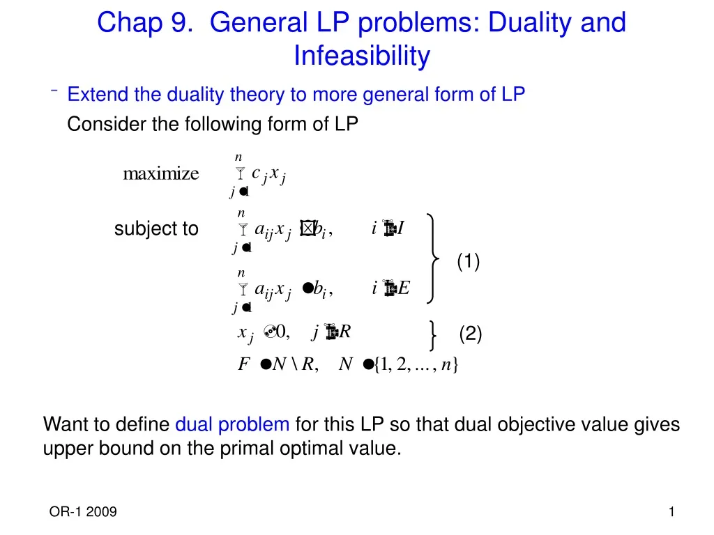
Chap 9. General LP problems: Duality and Infeasibility. Extend the duality theory to more general form of LP Consider the following form of LP. subject to. (1). (2). Want to define dual problem for this LP so that dual objective value gives upper bound on the primal optimal value.

E N D
Chap 9. General LP problems: Duality and Infeasibility • Extend the duality theory to more general form of LP Consider the following form of LP subject to (1) (2) Want to define dual problem for this LP so that dual objective value gives upper bound on the primal optimal value.
Take linear combination of constraints with multiplier yifor constraint i. yi 0 for i I , yiunrestricted in sign for i E doesn’t change the direction of the inequality. holds for x satisfying (1) and yi 0, i I, yi unrestricted i E. Want this as upper bound Compare this with primal obj. coeff. cj
Make We want strong bound, hence solve s. t. (Dual problem)
Primal-Dual Correspondence • Weak duality and strong duality relationship hold for general primal, dual pair. • We may convert the general primal problem to standard form, take dual, then simplify to get the same dual problem. (Another way to get dual for general LP)
If the LP is given in min form, we may convert it to max form and take its dual. Then converting the dual to max form gives the dual. Or we may find primal form, regarding the min form as dual problem and find dual of dual. • Ex) s. t. s. t. Dual problem is s. t.
Thm 9.1 (The Duality Theorem): If a linear programming problem has an optimal solution, then its dual has an optimal solution and the optimal values of the two problems coincide. Pf) proof parallels the idea for standard LP. At the termination of the simplex method, we identify dual vector y* from y’B = cB‘ and show that it is dual feasible and b’y* = c’x*.
Consider the special case of the general LP max c’x s.t. Ax = b x 0, which is used as standard LP problem by some people (maybe in minimization form). Its dual is min y’b s.t. y’A c’ y unrestricted • Suppose we solve the above primal problem using simplex method and find optimal basis B. Then the updated tableau is expressed the same way as we have seen before.
Here we don’t have slack variables appearing. • Since y is obtained from y’B = cB , the updated objective coefficients in the z-row can be regarded as cj – y’Aj for all basic and nonbasic variables. • At optimality, we have (cj – y’Aj ) 0, or y’Aj cj , hence y is dual feasible vector. The dual objective function value is y’b, which is the same value as the current primal objective function value cB’B-1b = cB’xB . Hence providing the proof that the current solution x is optimal to primal and y is optimal to dual respectively.
Unsolvable Systems of Linear Inequalities and Equations • Consider the following pair of constraints j=1n aijxj bi ( i I ) j=1n aijxj = bi ( i E ) yi 0 whenever i I i=1m aijyi = 0 for all j = 1, 2, … , n i=1m biyi < 0 • Then (9.13) is infeasible if and only if (9.16) is feasible. In other words, exactly one of (9.13) and (9.16) has a feasible solution. (called theorem of the alternatives, many other versions, very important tool and has many applications.) (9.13) (9.16)
Pf)) Suppose (9.16) has a feasible solution y. We multiply yi on both sides of constraints in (9.13) and add the lhs and rhs, respectively (with yi 0 for i I). Then, we obtain j=1n (i=1m aijyi ) xj i=1m biyi Hence, j=1n 0xj i=1m biyi < 0, which must be satisfied by any feasible x to (9.13). Since it is impossible to satisfy j=1n 0xj < 0 by any x, (9.13) is infeasible ) Consider the linear program max i=1m (-xn+i ) s.t. j=1n aijxj + wixn+i bi ( i I ) j=1n aijxj + wixn+i = bi ( i E ) xn+I 0 ( i = 1, 2, … , m) with wi = 1 if bi 0 and wi = -1 if bi < 0. (9.18) has a feasible solution (with x = 0 for original vars). Also the upper bound on optimal value is 0, hence it has finite optimal. (9.18)
(continued) The optimal value of (9.18) is 0 if and only if (9.13) has a feasible solution. If (9.13) is unsolvable, then the optimal value of (9.18) is negative. Then duality theorem guarantees that the dual of (9.18) has optimal value which is negative. min i=1m biyi s.t. i=1m aijyi = 0 ( j = 1, 2, … , n) wiyi -1 ( i = 1, 2, … , m) yi 0 ( i I ) Then the optimal dual solution y1, y2, … , ym satisfies (9.16)