Download
1 / 30
320 likes | 527 Views
Small Boat Attack in Malacca Straits. OA4202 Project Presentation. Chiam , Tou Wei (David) Lee, Kah Hock Nov 3, 2011. Background. Threat of Small Boats USS Cole Sea Tigers (LTTE) Gibraltar Plot. Why ? Fast and Maneuverable Narrow Sea Straits Heavy Shipping Traffic

E N D
Small Boat Attack in Malacca Straits OA4202 Project Presentation • Chiam, Tou Wei (David) • Lee, Kah Hock • Nov 3, 2011
Background • Threat of Small Boats • USS Cole • Sea Tigers (LTTE) • Gibraltar Plot • Why ? • Fast and Maneuverable • Narrow Sea Straits • Heavy Shipping Traffic • Sovereign Islands and Coasts 2
Problem for the Small Boat What is the best Starting Location & Minimum Risk Pathto attack a Naval Warshipalong Malacca Straits ? Terrorist Small Boat Malacca Straits Naval Warship 3
Assumptions • Warship is moving at constant speed, along a pre-determined route independent of small boat. • Small Boat Threat is aware of Warship locations at each point along its route. • Movement and Distances are based on the Manhattan convention. • As our project is unclassified, Data is generic and not based on actual operational systems. 4
Abstraction to Network Model Malacca Straits 9 Squares 10 Squares Channel of Interest : Width – 45 nm, Length – 50 nm Gridded Map : = 5 nm x 5 nm 5
Network Representation Time Step: 15 mins (5nm @ cruise speed of 20 kts) t + 30 mins t + 15 mins t mins Nodes – Position of Ships on Grid per time step Edges – Movement of Small Boat to next time step 6
Small Boat Movement Edges • Based on Speed : 1. Stationary or Loiter 3. Fast (40 kts) 2. Slow (20kts) • Based on Environment : • No Entry to Land Nodes • 2. Slow Speed upon entry, exit and within Shipping Lane 7
Edge Costs • Edge Cost = Reliability (0 to 1) • =1 - Risk (0 to 1) • Risk Components: • 1. Exposure Risk – Environmental Cover • 2. Proximity Risk – Distance to Warship • 3. LOS Risk – Line-of-Sight with Warship • Total Edge Risk = • [(We* Exposure Risk) + (Wp* Proximity Risk)] * LOS Risk • We,Wp: Normalised weights for multi-objective risk assessment • (currently set to be equal, 0.5) 8
Risk Assignment • Exposure Risk • Proximity Risk • Within LOS Risk Factor = 0.8 9
Minimum Risk to Shortest Path LP • Minimum Risk Path = Maximum Reliability Path • = Max • = - Min • LP Formulation : • a,i,j :position nodes at each time step • s: start node to all small boat positions at time step 0 • t:end node from all warship positions • rij: reliability (in –ve log terms) of edge from node i to j • yij:1 - if edge from node i to j is in shortest path, 0 - otherwise 10
Attacks on the Network • Surveillance Points on Grid • - Coastal Radars, Cameras • - Escorts • - Patrol Aircraft • Surveillance Effects • - Edge Level: Reduces Reliability of a single edge • - Node Level: Reduces Reliability of all incoming edges 11
Maximize Attack Effects • Max-Min LP Formulation • a,i,j :position nodes at each time step • s:start node to all small boat positions at time step 0 • t:end node from all warship positions • cij: reliability(in –ve log terms) of edge from node i to j • yij:1 - if edge from node i to j is in shortest path, 0 – otherwise • sij: surveillance effect on safety edge cost from node i to j • xij: 1 - if edge from node i to j is under surveillance, 0 – otherwise 12
Max-Min conversion for GAMS • Apply Dual Formulation, into a GAMS-friendly MIP • (Node-level surveillance) • i,j:position nodes at each time step • s: start node to all small boat positions at time step 0 • t:end node from all warship positions • i: minimum reliability (in –ve log terms) from start node to node i • cij: reliability (in -ve log terms) of edge from node i to j • sij: surveillance effect on safety edge cost from node i to j • xi: 1 - if node i is under surveillance, 0 – otherwise • xij: 1 - if edge from node i to j is under surveillance, 0 – otherwise 13
Results: Fixed Start Locations C C A A B B D D 14
Results: Any Start Location Shipping Lanes B – Small Boat Path Exploits Shipping Lanes and Coast for cover – Warship Path – Seawater – Coastal Land Takes most Direct Route to Warship as she comes Minimal Risk Path starts near to Warship 15
Surveillance Effects on Path Edge Blocking Node Blocking B – Small Boat – Incoming Edge Blocked W– Warship Path – Destination Node Blocked 16
Node Blocking Trends SP=0 SP=1 SP=2 SP=3 SP=4 SP=5 SP=6 SP=7 SP = # Surveillance Points 17
Node Degradation Trends SP=0 SP=1 SP=2 SP=3 SP=4 SP=13 SP=14 SP=15 SP = # Surveillance Points 18
Operator Resilience Curves SP=2 SP=3 3: All nearby paths with Shipping Lanes and Coast Cover are blocked 5-7: Minimal Changes in Path Direction 8-11: Projected to Completely Block at 11. 19
Operator Resilience Curves SP=5 SP=6 SP=7 3: All nearby paths with Shipping Lanes and Coast Cover are blocked 5-7: Minimal Changes in Path Direction 8-11: Projected to Completely Block at 11. 20
Operator Resilience Curves SP=7 3: All nearby paths with Shipping Lanes and Coast Cover are blocked 5-7: Minimal Changes in Path Direction 8-11: Projected to Completely Block at 11. 21
Operator Resilience Curves SP=2 SP=3 SP=0 3: Path crosses a SP 14: All possible degradation Nodes covered in Direct Path to Warship 22
Operator Resilience Curves SP=14 SP=15 SP=0 3: Path crosses a SP 14: All possible degradation Nodes covered in Direct Path to Warship 23
Mixture of Surveillance Assets • Consider 2 types of assets: • Small Area • Influences arcs connecting nearest neighbor • Penalty 50% • Large Area • Influences arcs connecting up to 2 nodes away • Less effective than short range (Penalty 20%) 24
Mixture of Surveillance Assets 9 • From 3 assets onwards, Small Area asset has more impact 25
Mixture of Surveillance Assets • Large Area asset complements limitation of Small Area asset 26
If we had more time… • Potential Enhancements • Interdiction represented by path in time (Persistence) • Mixture of “Area” and “Directional” influence assets • Costs of assets, subject to budget • Concurrent attempt by more than 1 boat 28
Computational Complexity • # Nodes : • - Length (10) x Width (9) x Time Steps (13) = 1170 • - With Start, End Nodes & Inaccessible Land Nodes = 847 • # Edges : • - Moves per node = Stationary(1) + Slow(4) + Fast (8) = 13 • - # Nodes x Moves per node = 10895 • - With Start, End Nodes and Prohibited Moves = 5698 • General LP : • O(big x small2) = O(n x m2) • MIP : • O(# branch iterations x (n x m2)) 30