Download
1 / 33
330 likes | 351 Views
Phononless AC conductivity in Coulomb glass. Jacek Matulewski, Sergei Baranovski, Peter Thomas Departament of Physics Phillips-Universitat Marburg, Germany Faculty of Physics, Astronomy and Informatics Nicolaus Copernicus University in Toruń, Poland R á ckeve, 30 VIII 2004.

E N D
Phononless AC conductivity in Coulomb glass Jacek Matulewski, Sergei Baranovski, Peter Thomas Departament of Physics Phillips-Universitat Marburg, Germany Faculty of Physics, Astronomy and Informatics Nicolaus Copernicus University in Toruń, Poland Ráckeve, 30 VIII 2004 Monte-Carlo simulations
Outline 1. Experimental results of AC conductivity measurements 2. Shklovskii and Efros’s model of zero-phonon AC hopping conductivity in the disordered system 3. “Coulomb term” 4. Simulation procedure 5. Results a) Coulomb gap in states distribution b) Pairs distribution c) Conductivity
Experimental results M. Lee and M.L. Stutzmann, Phys. Rev. Lett. 87, 056402 (2001) E. Helgren, N.P. Armitage and G. Gru:ner, Phys. Rev. Lett. 89, 246601 (2002)
Experimental results M. Lee and M.L. Stutzmann, Phys. Rev. Lett. 87, 056402 (2001) E. Helgren, N.P. Armitage and G. Gru:ner, Phys. Rev. Lett. 89, 246601 (2002)
Outline 1. Experimental results of AC conductivity measurements 2. Shklovskii and Efros’s model of zero-phonon AC hopping conductivity in the disordered system 3. “Coulomb term” 4. Simulation procedure 5. Results a) Coulomb gap in states distribution b) Pair distribution c) Conductivity
Shklovskii and Efros’s model of zero-phonon AC hopping conductivity of disordered system System of randomly distributed sites with Coulomb interaction: Electron-electron interactions are taken into account! Site energy: (sites are identical) • When T 0K, the Fermi level is present • If frequency of external AC electric field is small, only pairs near the Fermi level contribute to conductivity (one site below and one over) • Pair approximation
Overlap of site’s wavefunction Site energy is determined by Coulomb interaction with surrounding pairs Notice that because of overlap I(r) “intuitive” states can be not good eigenstates Anyway four states are possible a priori: • there is no electron, so no interaction and energy is equal to 0 • there is one electron at the pair (two states) • there are two electrons at the pair Shklovskii and Efros’s modelPair of sites Hamiltonian of a pair of sites:
The isolated sites base Normalisation where Shklovskii and Efros’s modelPair of sites Only pairs with one electron are interesting in context of conductivity:
Source of energy: photons Energy which must be absorbed by pairs in unit volume due to change states prob. of finding “proper” pair prob. of finding photon with energy equals to · QM transition prob. (Fermi Golden Rule) · · Q = Shklovskii and Efros formula for conductivity in Coulomb glasses And finally the conductivity: Numerical calculation (esp. for T > 0) Shklovskii and Efros’s modelPair of sites Energy which pair much absorb or emit to move the electron between split-states(from to ): Two limits
Outline 1. Experimental results of AC conductivity measurements 2. Shklovskii and Efros’s model of zero-phonon AC hopping conductivity in the disordered system 3. “Coulomb term” 4. Simulation procedure 5. Results a) Coulomb gap in states distribution b) Pair distribution c) Conductivity
Additional Coulomb energy in transition Correction to sites energy difference
+ + In order to make the calculation possible we need to express the energy difference using sites energy values before the transition Additional Coulomb energy in transition Dj Site energies Energy of the system: Di A (all acceptors)
Additional Coulomb energy in transition • Physical cause of correction: changes in the Coulomb net configuration • Pair approximation: only one pair changes the state at the time • Unfortunately to obtain this term we need to forget about the overlap for a moment In order to make the calculation possible we need to express the energy difference using sites energy values before the transition
Outline 1. Experimental results of AC conductivity measurements 2. Shklovskii and Efros’s model of zero-phonon AC hopping conductivity of disordered system 3. “Coulomb term” 4. Simulation procedure a) T = 0K (Metropolis algorithm) b) T > 0K (Monte-Carlo simulation) 5. Results a) Coulomb gap in states distribution b) Pair distribution c) Conductivity
Simulation procedure (T = 0K) Metropolis algorithm: the same as used to solve the milkman problem General: Searching for the configuration which minimise some parameter In our case: searching for electron arrangement which minimise total energy N=10K=0.5 Occupied donor Empty donor Occupied acceptor
Step 01. Place N randomly distributed donors in the box2. Add K·N randomly distributed acceptors Step 1 (m -sub)3. Calculate site energies of donors4. Move electron from the highest occupied site to the lowest empty one 5. Repeat points 3 and 4 until there will be no occupied empty sites below any occupied (Fermi level appears) Simulation procedure (T = 0K) Metropolis algorithm for searching the pseudo-ground state of system
Step 2 (Coulomb term)6. Searching the pairs checking for occupied site j and empty i If there is such a pair then move electron from j to iand call m -sub (step 1) and go back to 6. Effect: the pseudo-ground state (the state with the lowest energy in the pair approximation) • Energy can be further lowered by moving two and more electrons at the same step (few percent) Simulation procedure (T = 0K) Metropolis algorithm for searching the pseudo-ground state of system Dlaczego nie gamma?????
Simulation procedure (T > 0K) Monte-Carlo simulations Step 3 (Coulomb term)7. Searching the pairs checking for occupied site j and empty i If there is such a pair Then move electron from j to i for sureElse move the electron from j to i with prob. Callm -sub (step 1). Repeat step 3 thousands times Repeat steps 0-3 several thousand times (parallel)
Outline 1. Experimental results of AC conductivity measurements 2. Shklovskii and Efros’s model of zero-phonon AC hopping conductivity in the disordered system 3. “Coulomb term” 4. Simulation procedure 5. Results a) Coulomb gap in states distribution b) Pair distribution c) Conductivity
Coulomb gap in density of states for T = 0K Coulomb gap created due to Coulomb interaction in the system Coulomb term, but not only ... Si:P Normalized single-particle DOS
10000 T = 0 (0K) T = 0.3 (725K) 9000 T=1 (2415K) 8000 7000 6000 5000 4000 3000 2000 1000 0 -4 -2 0 2 4 Smearing of the Coulomb gap for T > 0K Normalized single-particle DOS
Pair distribution (T = 0K) N=400, T=0K, NMonte-Carlo=1000, a=0.27
Pair distribution (T > 0K) N=400, T=1/8 (300K), NMonte-Carlo=1000, a=0.27
Pair distribution (T > 0K) N=400, T=1 (2415K), NMonte-Carlo=1000, a=0.27
pair mean spatial distance simulations Mott’s formula Pairs mean spatial distance (T = 0K) N=1000, K=0.5, 2500 realisations periodic boundary conditions, AOER Distribution of pairs’ distances is very wide in contradiction to Mott’s assumption
250000 200000 150000 100000 50000 0 0 1 2 3 4 5 6 7 8 9 10 Pair energy distribution (T = 0K) N=500, T=0, K=0.5, aver. over 100 real. Number of pairs We work here!!!
Conductivity (T=0K) N=500, T=0, K=0.5, aver. over 25k real. Δ(hw)=0.001 (blue), Δ(hw)=0.01 (green) Helgren et al. (T=2.8K) n = 69% simulations Conductivity (arb. un.) fixed parameters for Si:P: a = 20Å, and nC = 3.52·1024 m-3 (lC = 65.7Å) n = 69% of nC means a = 0.27 [l69%] (in units of n-1/3) There is no crossover in numerical results!
Conductivity (T=0K) N=500, T=0, K=0.5, aver. over 25k real. Δ(hw)=0.001 (blue), Δ(hw)=0.01 (green) 0.0001 simulations Helgren 69% Si:P 1e-005 clearly visible crossover Conductivity (arb. un.) 1e-006 1e-007 a = 0.36 1e-008 0.001 0.01 0.1
250000 T = 0 T = 0.125 200000 T = 0.3 T = 0.5 T = 1 150000 100000 50000 0 0 0 0.5 0.5 1 1 1.5 1.5 2 2 2.5 2.5 3 3 Number of pairs for T > 0K N=500, T=0, K=0.5, aver. over 100 real. Number of pairs
0.0005 T = 0.0 0.00045 T = 0.1 T = 0.5 0.0004 T = 1.0 0.00035 0.0003 0.00025 0.0002 0.00015 0.0001 5e-005 0 0 0.05 0.1 0.15 0.2 0.25 0.3 Conductivity for T > 0K N=500, T=0, K=0.5, aver. over 1000 real. Δ(hw)=0.01, T>0 Conductivity (arb. un.)
w = 0.001 w = 0.01 w = 0.1 (0.5·1013 Hz) Conductivity for T > 0K N=500, T=0, K=0.5, aver. over 1000 real. Δ(hw)=0.01, T>0 Si:P 69% Conductivity (arb. un.) temperature (dimensionless units)
fitting of (Baranovskii et al.) fitting of (Efros) Shape of Coulomb gap for T = 0K (corresponding to conductivity in low frequency) numerical simulations result Normalized single particle-DOS this hump probably is only a model artefact Efros: many particle-hole excitations in which surrounding electrons were allowed to relax hard gap