Download
1 / 41
410 likes | 523 Views
Gravitational Energy: a quasi-local, Hamiltonian approach . Jerzy Kijowski Center for Theoretical Physics PAN Warsaw, Poland. In most cases the Cauchy problem is „well posed” due to the existence of a positive, local energy. Example 1: The (non-linear) Klein-Gordon field:.

E N D
Gravitational Energy:a quasi-local, Hamiltonian approach Jerzy Kijowski Center for Theoretical Physics PAN Warsaw, Poland
In most cases the Cauchy problem is „well posed” due to the existence of a positive, local energy. Example 1: The (non-linear) Klein-Gordon field: where is the momentum canonically conjugate to the field variable ; (linear theory for ). Example 2: Maxwell electrodynamics: where – electric and magnetic field. Energy estimates in field theory Field energy, if positive, enables a priori estimations. ROAD TO REALITY, Warsaw
energy-momentum tensor conservation laws: relativistic invariance Indeed: gravitational energy cannot be additive because of gravitational interaction: Gravitational energy In special relativity field energy obtained via Noether theorem: But: no energy-momentum tensor of gravitational field! No space-time symmetry or too many symmetries! Various „pseudotensors” have been proposed. They do not describe correctly gravitational energy! ROAD TO REALITY, Warsaw
Boundary integrals vanish. Volume integrals carry information. Volume integrals vanish. Boundary integrals carry information. Bulk versus boundary Standard „Hamiltonian” approaches to special-relativistic field theory is based on integration by parts and neglecting surface integrals at infinity („fall of” conditions). Paradigm: functional-analytic framework for description of Cauchy data must be chosen in such a way that the boundary integrals vanish automatically! Trying to mimick these methods in General Relativity Theory we painfully discover the opposite rule: General relativity: strong „fall off” conditions trivialize the theory. ROAD TO REALITY, Warsaw
Gravitational energy contained in a three-volume has to be assigned to its boundary . ( instead of ) R. Penrose (1982, 83) proposed a quasi-local approach: Gravitational energy asigned to closed 2D surfaces. Quasi-local approach Meanwhile, many (more than 20) different definitions of a „quasi-local mass” (energy) have been formulated. In this talk I want to discuss a general Hamiltonian framework, where boundary integrals are not neglected! This approach covers most of the above 20 different definitions: each related to a specific „control mode”. ROAD TO REALITY, Warsaw
Symplectic space : a manifold equipped with a non-degenerate, closed differential two-form . Basic example: co-tangent bundle of a certain „configuration space” . Cotangent bundle carries a canonical one-form: where are coordinates in and are the corres- ponding „canonical coordinates” in the co-tangent bundle. Symplectic relations We begin with a mathematical analysis of energy as a generator of dynamics in the sense of symplectic relations. ROAD TO REALITY, Warsaw
Any function on the base manifold generates a Lagrangian (i.e. maximal, isotropic for ) submanifold of the co-tangent bunle, according to the formula: Every lagrangian submanifold which is transversal with respect to fibers of the bundle is of that type, i.e. has a generating function. Also non-transversal manifolds can be described this way in a slightly broader framework (constraints, Morse functions). Generating function ROAD TO REALITY, Warsaw
Thermodynamical properties of a simple body can be encoded by the following formula: The proper arena for describing these properties is a four-dimensional phase space (pressure, temperature, volume and entropy). This „meta-phase space” is equipped with the („God given”) symplectic structure: describing any simple thermodynamical body. A specific body is described by a specific generating function , as a two-dimesional submanifold satisfying equations: Energy as a generating function ROAD TO REALITY, Warsaw
Interpretation: have been chosen as „configuration” or „control parameters”, whereas are „momenta” or „response parameters”. The same submanifold (collection of all physically admissible states) can be described by the Helmholz free energy function, via the formula: The same physics, but different control modes Energy as a generating function ROAD TO REALITY, Warsaw
Energy as a generating function Legendre transformation: transition from one control mode to another: ROAD TO REALITY, Warsaw
The (4N-dimensional) „meta- phase space” describes: positions , velocities , momenta , and forces . Equipped with the canonical („God given”) symplectic form: Mechanics: variational formulation Euler-Lagrange equation in classical mechanics, together with the definition of canonical momenta may be written as: ROAD TO REALITY, Warsaw
The Hamiltonian function The same physics, different control modes Mechanics: Hamiltonian formulation ROAD TO REALITY, Warsaw
Consider scalar field theory derived from a variational principle: Field equations can be written in the following way: At every spacetime point we have a 10-dimensional symplectic „meta-phase space” describing: field strength , its 4 derivatives , corresponding 4 momenta , and their divergence . - exterior derivative within this space („vertical” in contrast to spacetime derivatives)! Scalar field theory ROAD TO REALITY, Warsaw
Consider scalar field theory derived from a variational principle: Field equations can be written in the following way: At every spacetime point we have a 10-dimensional symplectic „meta-phase space” describing: field strength , its 4 derivatives , corresponding 4 momenta , and their divergence . Symplectic structure give by: Submanifold : field equations. Scalar field theory ROAD TO REALITY, Warsaw
Consider scalar field theory derived from a variational principle: Field equations can be written in the following way: Hamiltonian formulation: based on a (3+1) decomposition. Scalar field theory The formalism is coordinate-invariant. Partial derivatives can be organized into invariant geometric objects: jets of sections of natural bundles over spacetime. ROAD TO REALITY, Warsaw
Consider scalar field theory derived from a variational principle: Scalar field theory Field equations can be written in the following way: index „k=1,2,3” denotes three space-like coordinates, index „0” denotes time coordinate. We denote . Hamiltonian formulation: based on a (3+1) decomposition. ROAD TO REALITY, Warsaw
Consider scalar field theory derived from a variational principle: Standard „Legendre manipulations” give us: Scalar field theory Field equations can be written in the following way: index „k=1,2,3” denotes three space-like coordinates, index „0” denotes time coordinate. We denote . ROAD TO REALITY, Warsaw
Integrating energy density over a 3-volume V we obtain: - transversal to boundary component of the momentum amount of energy contained in V Infinite-dimensional Hamiltonian system Scalar field theory Energy generates dynamics as a relation between three objects: initial data, their time derivatives and the boundary data. Field dynamics within V can be made unique (i.e Cauchy problem „well posed”) if we impose boundary conditions annihilating the boundary term. ROAD TO REALITY, Warsaw
Another way to kill the boundary term: fix Neuman data : They are generated by two different Hamiltonians: or . adiabatic insulation? Scalar field theory Both evolutions are equally legal. Which one is the field’s „true energy”? ROAD TO REALITY, Warsaw
Dirichlet data fixed at the boundary Neuman data fixed at the boundary free energy energy; can also be obtained from energy-momentum tensor Dirichlet vs. Neuman evolution ROAD TO REALITY, Warsaw
Classical elecrodynamics (also non-linear, like Born-Infeld) can be derived from a variational principle: Variation with respect to the electromagnetic potential . Linear Maxwell theory if: Standard (texbook) procedure leads to the „canonical” en-mom. tensor and the corresponding „canonical” energy . Adding a boundary term one can construct the „symmetric” en-mom. tensor and the corresponding „symmetric” energy . Electrodynamics ROAD TO REALITY, Warsaw
It can be proved that „symmetric energy” generates a Hamiltonian field evolution based on controlling magnetic and electrix flux at the boundary : For linear Maxwell theory we have: But: „canonical energy” (usually claimed to be „unphysical”) generates an equally good Hamiltonian field evolution based on controlling magnetic flux and electostatic potential at . Electrodynamics ROAD TO REALITY, Warsaw
grounding plug adiabatic insulation generator : free energy generator : true energy Energy vs. free energy Different control modes at the boundary: ROAD TO REALITY, Warsaw
Field configuration described by two 3-dimesional vectors: B, D. Dynamics given by Maxwell equations: wave operator Consider two functions describing radial components of D and B. Hence, Maxwell equations imply: Dirichlet vs. Neuman in Electrodynamics A „flavour of the proof” for linear Maxwell theory. ROAD TO REALITY, Warsaw
These are the only two dynamical equations. Initial data: carry entire information about fields In spherical coordinates electric fields is decomposed as follows: Radial component is directly encoded by the function . ( - angular coordinates.) On each sphere the tangent part can be further decomposed into a sum of a gradient and co-gradient: The co-gradient part can be reconstructed from : Dirichlet vs. Neuman in Electrodynamics ROAD TO REALITY, Warsaw
The gradient part can be reconstructed from the constraint equation , namely: Quasi-local reconstruction: on each sphere separately. Dirichlet control mode for both and : control of and . Generator: „symmetric energy” . True energy Neuman control mode for and Dirichlet for : control of and . Generator: „canonical energy” . Free energy Dirichlet vs. Neuman in Electrodynamics ROAD TO REALITY, Warsaw
1) metric (variation with respect to ). 2) Palatini (variation with respect to both and treated as independent fields). 3) affine (variation with respect to , metric arises as a momentum conjugate to connection). General relativity theory Gravitational field equations – Einstein equations. Can be derived from various variational formulations: Examples: Hamiltonian theory based on (3+1) decomposition is universal and does not depend upon a particular variational formula. Cauchy data on a hypersurface: 3-metric and exterior curvature. ROAD TO REALITY, Warsaw
Arnowitt-Deser-Misner momentum (1962): We expect Hamiltonian formula of the type: Non-unique ! (boundary manipulations) expected: quasi-local unknown boundary control Bulk term – due to ADM. General relativity theory ROAD TO REALITY, Warsaw
can be obtained directly from Time derivatives Einstein equations (e.g.: WMT, page 525). Pluging these quantities into the bulk term, we can calculate directly the remaining boundary terms. General relativity theory No variational formulation necessary! ROAD TO REALITY, Warsaw
General relativity theory ROAD TO REALITY, Warsaw
Geometry of T in (2+1) – decomposition. Gauge invariant canonical phase space form. Now invariant! Non-invariant! Fundamental identity ROAD TO REALITY, Warsaw
Gauge transformation: Fundamental identity Now invariant! ROAD TO REALITY, Warsaw
This is not a control mode because are not independent! Analogous to 4D phase space of the particle dynamics: Fundamental identity ROAD TO REALITY, Warsaw
Given a 2D surface S, choose the tube T. Natural choice: Fundamental identity ROAD TO REALITY, Warsaw
Fundamental identity ROAD TO REALITY, Warsaw
Fundamental identity Examples: 1) „Metric control mode” – complete metric of T is controlled. ROAD TO REALITY, Warsaw
Fundamental identity Examples: 2) „Mixed control mode” – only 2D metric of S and time-like components of Q controlled. ROAD TO REALITY, Warsaw
Fundamental identity ROAD TO REALITY, Warsaw
Generic 2D-surface S carries a natural „time” and „space” directions. Control of is natural. Conclusions Fundamental formula – natural framework for quasi-local analysis of gravitational energy. Valid also for interacting system: „matter fields + gravity” (if supplemented by appropriate matter terms in both the Hamiltonian and the control parts). ROAD TO REALITY, Warsaw
Generic 2D-surface S carries a natural „time” and „space” directions. Control of is natural. Conclusions Any choice of the remaining control leads to a „quasi-local energy. Which one is „the true energy” and not a „free energy”? Criteria: positivity, „well posedness”, linearization ... ROAD TO REALITY, Warsaw
Example: Klein-Gordon theory. Standard Lagrangian density: Exchanging role of the field and the momentum we may derive the same theory from the following variational principle: Scalar field theory Boundary terms added to the Lagrangian are irrelevant! Both Lanrangians differ by a boundary term. They define the same field equations. Choosing either Dirichlet or Neuman control mode we get different Hamiltonian systems. ROAD TO REALITY, Warsaw