The Search for Gravitational Waves using Pulsar Timing

1. The Search for Gravitational Waves using Pulsar Timing R. N. Manchester CSIRO Astronomy and Space Science Sydney Australia Summary • Brief introduction to pulsars and timing • Detection of GW using pulsar timing • Pulsar Timing Array (PTA) projects • Current status and future prospects

2. What are pulsars? • Pulsars are rotating neutron stars radiating beams of emission that we see as pulses as they sweep across the Earth • Neutron stars are formed in supernova explosions by the collapse of the core of a massive star • Millisecond pulsars are old neutron stars that have been recycled by accretion of matter from a binary companion • Almost all known pulsars lie within our Galaxy • Neutron stars have a mass about 1.4 MSun but a radius of only ~15 km • Their surface gravity is enormous, ~1012gEarth, hence their break-up rotation speed is very high, ~1 kHz

3. A Pulsar Census • Currently 2405 known (published) pulsars • 2162 rotation-powered Galactic disk pulsars • 243 in binary systems • 353 millisecond pulsars • 142 in globular clusters • 8 X-ray isolated neutron stars • 21 magnetars (AXP/SGR) • 28 extra-galactic pulsars Data from ATNF Pulsar Catalogue, V1.52 (www.atnf.csiro.au/research/pulsar/psrcat) (Manchester et al. 2005)

4. Pulsars as Clocks • Because of their large mass and small radius, NS spin rates - and hence pulsar periods – are extremely stable • For example, in 2001, PSR J0437-4715 had a period of : 5.757451924362137 +/- 0.000000000000008 ms • Although pulsar periods are very stable, they are not constant • Pulsars are powered by their rotational kinetic energy • They lose energy to relativistic winds and low-frequency electromagnetic radiation (the observed pulses are insignificant) • Consequently, all pulsars slow down (in their reference frame) • Typical slowdown rates are less than a microsecond per year • For millisecond pulsars, slowdown rates are ~105 smaller

5. Measurement of pulsar periods • Start observation at a known time and average 103 - 105 pulses to form a mean pulse profile • Cross-correlate this with a standard template to give the arrival time at the telescope of a fiducial point on profile, usually the pulse peak – the pulse time-of-arrival (ToA) • Measure a series of ToAsover days – weeks – months – years • Transfer ToAsto an inertial frame – the solar-system barycentre • Compare barycentricToAswith predicted values from a model for the pulsar – the differences are called timing residuals. • Fit the observed residuals with functions representing errors in the model parameters (pulsar position, period, binary period etc.). • Remaining residuals may be noise – or may be science!

6. Sources of Pulsar Timing “Noise” • Intrinsic noise • Period fluctuations, glitches • Pulse shape changes • Perturbations of the pulsar’s motion • Gravitational wave background • Globular cluster accelerations • Orbital perturbations – planets, 1st order Doppler, relativistic effects • Propagation effects • Wind from binary companion • Variations in interstellar dispersion • Scintillation effects Pulsars are powerful probes of a wide range of astrophysical phenomena • Perturbations of the Earth’s motion • Gravitational wave background • Errors in the Solar-system ephemeris • Clock errors • Timescale errors • Errors in time transfer • Instrumental errors • Radio-frequency interference and receiver non-linearities • Digitisation artifacts or errors • Calibration errors and signal processing artifacts and errors • Receiver noise

7. . The P – P Diagram Galactic Disk pulsars P = Pulsar period P = dP/dt = slow-down rate . . • For most pulsars P ~ 10-15 • MSPs haveP smaller by about 5 orders of magnitude • Most MSPs are binary, but few normal pulsars are • τc = P/(2P) is an indicator of pulsar age • Surface dipole magnetic field ~ (PP)1/2 . . . Great diversity in the pulsar population! (Data from ATNF Pulsar Catalogue V1.50)

8. Pulsars and Gravitational Waves • Pulsars have already shown that GW exist • Double-neutron-star systems emit GW at 2forb • Energy loss causes slow decrease of orbital period • Predict rate of orbit decay from known orbital parameters and NS masses using GR • For PSR B1913+16, ratio of measured value to predicted value = 0.997 +/- 0.002 PSR B1913+16 Orbit Decay • First observational evidence for gravitational waves! (Weisberg , Nice & Taylor 2010)

9. The Double Pulsar PSR J0737-3039A/B R: Mass ratio w: periastron advance g: gravitational redshift r & s: Shapiro delay Pb: orbit decay WSO: Spin-orbit coupling . • Six measured relativistic parameters(!) + mass ratio • Five independent tests of GR • Now limits deviations from GR to 0.02% • Pb,GW now more precise than for PSR B1913+16 . (Kramer et al. 2015)

10. Pulsar Timing Arrays (PTAs) • A PTA consists of many pulsars widely distributed on the sky with frequent high-precision timing observations over a long data span • Can in principle detectgravitational waves (GW) • GW passing over the pulsars are uncorrelated • GW passing over Earth produce a correlated signal in the TOA residuals for all pulsars • Most likely source of GW detectable by PTAs is a stochastic background from super-massive binary black holes in distant galaxies • PTAs are sensitive to long-period GWs, fGW ~ 1/(data span) ~ few nanohertz–complementary to laser-interferometer systems • Detection requires precision timing of ~20 MSPs over ~10 years • PTAs can also detect instabilities in terrestrial time standards – establish a pulsar timescale Idea first discussed by Hellings & Downs (1983), Romani (1989) and Foster & Backer (1990)

11. Correlated Timing Signals • Clock errors All pulsars have the same TOA variations: Monopolesignature • Solar-System ephemeris errors Dipole signature • Gravitational waves Quadrupolesignature Hellings & Downs GW correlation function Can separate these effects provided there is a sufficient number of widely distributed pulsars (Hobbs et al. 2009)

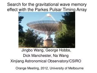
12. Major Pulsar Timing Array Projects • European Pulsar Timing Array (EPTA) • Radio telescopes at Westerbork, Effelsberg, Nancay, Jodrell Bank, Cagliari • Timing ~40 MSPs, 5 - 18 years (Kramer & Champion 2013) • North American pulsar timing array (NANOGrav) • Data from Arecibo and Green Bank Telescope • Timing ~30 MSPs, data spans 3 - 28 years (McLaughlin 2013) • Parkes Pulsar Timing Array (PPTA) • Data from Parkes 64m radio telescope in Australia • Timing 22 MSPs, data spans 3 – 19 years (Manchester et al. 2013)

13. MSPs suitable for PTAs All (published) MSPs not in globular clusters

14. PPTA Three-Band Timing Residuals 50cm • Regular observations in three bands: 50cm ~700 MHz 20cm ~1400 MHz 10cm ~3100 MHz • Frequency-dependent variable delays: due to dispersion variations resulting from ISM density fluctuations • Delay Δt ~ ν-2 10cm 20cm (Manchester et al. 2013)

15. PPTA Timing Residuals (DR1) • Timing data for 22 pulsars • Data spans to 19 years • Best 1-year rms timing residuals about 40 ns, most < 1μs • Low-frequency (red) variations significant in about half of sample – some due to uncorrected DM variations in early data, e.g., J1045-4509 • Some of the best-timing pulsars nearly white (e.g., J1713+0747, J1909-3744) (Hobbs 2013)

16. Effect of GW on pulsar timing residuals Redshift z of observed pulsar frequency is difference between the effects of GW passing over the pulsar and the GW passing over the Earth: where the GW is propagating in the +z direction and α, β, γ are direction cosines of the pulsar from Earth. is the difference in GW strains at the pulsar and the Earth (A = polarisation). is the “pulsar term” (d is the pulsar distance) and is the “Earth term”. The observed timing residuals are the integral of the net redshift: (Detweiler 1979, Anholm et al. 2009)

17. Pulsar timing “antenna pattern” • Timing response is maximum for a pulsar (roughly) in the direction of the GW source • Response is zero for pulsars exactly in both source and propagation direction • For different pulsars of a PTA, the pulsar terms are uncorrelated, both because of the retarded time and the different GW environment, but the Earth terms are correlated. • For an isotropic GW background, many different GW sources – have to integrate antenna pattern over different GW propagation directions • Hellings & Downs (1983) showed that the correlated Earth-term response was a function only of the angle θ between pulsars: z GW source  (Chamberlin & Siemens 2012) where • Uncorrelated pulsar term produces “noise” on HD curve

18. The Isotropic GW Background • Strongest source of nHz GW waves is likely to be a background from orbiting super-massive black holes in distant galaxies Rate of energy loss to GW: Chirp mass: Frequency in source frame: • Number of mergers per co-moving volume based on model for galaxy evolution (e.g. Millennium simulation) plus model for formation and evolution of SMBH in galaxies (Sesana 2013)

19. Simple parameterisation of characteristic strain for cosmological distribution of circular BH binaries: A is the characteristic strain at a GW frequency f = 1/(1 yr) • GW modulates the observed pulsar frequency • Modulation spectrum of observed timing residuals: GW power ~ f -13/3 • Spectrum is very steep – Cholesky spectral estimation methods needed to avoid leakage (Coles et al. 2011) • Strength of GWB often expressed as a fraction of closure energy density of the Universe: (Phinney 2001; Jenet et al. 2006)

20. Distribution of SMBBH contributing to the GWB • Most of background from SMBBH in galaxies at z = 1 – 2 • Biggest contribution from largest BH masses: 108 – 109Msun (Sesana et al. 2008)

21. PPTA Limit – Shannon et al. 2013 95% Confidence Limits • Based on six best PPTA pulsars + archival Arecibo data for one pulsar • Data spans 5 – 25 years – effective fGW ~ 2.8 nHz • 95% confidence limit based on detection statistic + simulations with GWB injection: Probability of a GW signal in the PPTA data (Milleniumsim) Hydro sim. (Kuiler et al. 2013) (Sesana 2013) (McWilliams et al. 2012) A< 2.4 x 10-15 Ωgw(fGW) < 1.3 x 10-9 (Shannon et al., 2013, Science)

22. Single Sources • Likely that many SMBH binary systems are highly eccentric • GW spectrum may be dominated by a strong individual source First GW detection by PTAs could be a single source with period <~ 1 year! (Sesana 2012)

23. PPTA Limits on Single GW Sources • Searched PPTA data set for arbitrary time series of GW amplitudes A+, Ax that satisfy the quadrupolar constraints for a given source direction • Searched these time series for sinusoidal components that could result from orbital motion of a SMBHB • Repeated for all possible source directions 2 yr-1 1 yr-1 Distance (Mpc) to which a SMBBH with chirp mass 109MSun emitting GW at 10-8 Hz can be detected Spectral strain sensitivity at different sky locations (Zhu et al. 2014)

24. Localisation of a GW Source • PPTA data set • Simulated source in Fornax cluster, S/N ~ 5 (100 ns amplitude) • Correlation statistic, Earth term only • Max detection statistic (o) close to source position • Localisation poor ~ 400 sqdeg (Zhu et al. (2015) • In principle, could make use of pulsar term as well – pulsar-Earth interferometer • Fringe spacing θf = λGW/[2πd(1+γ)] – few arc minute (γis zdirection cosine) • Localisation ~ θf/(S/N) – sub-arc-min possible • However, pulsar distances must be known to better than λGW/(1+γ) • So far, only one pulsar (J0437-4715) has sufficiently accurate dist. (d = 156.79±0.25 pc) (Reardon et al. 2015) (Lee et al. 2011)

25. GW “Memory” Events • Coalescence of two super-massive black holes creates an offset in space-time which propagates away at the speed of light • When such an offset crosses the pulsar or the Earth it causes a step frequency change (glitch) in the observed pulsar period • Events crossing the Earth have the same quadrupolar signature as a normal GW and so can be detected using similar techniques • PPTA data set used to limit amplitude and rate of GWM events • Long way from predictions! • Detection will take 50 MSPs, 50ns ToA precision, 25 yr data span – needs FAST and SKA PPTA data set 20-yr “PPTA” data set Predictions based on GWB models (Wang et al. 2014)

26. A New Limit on the Nanohertz GW Background • Based on PPTA 10cm data sets for the four best-timed pulsars • 11-year data span – 3.5 yrs longer than Shannon et al. (2013) PPTA data set • Inclusion of 20cm and 50cm data reduces the sensitivity – DM corrections are not sufficiently accurate Also fixed some small instrumental phase jumps • Bayesian analysis method • New limit: A < 1.0 x 10-15 • ΩGW < 2.3 x 10-10at f = 0.2 yr-1 (6 nHz) J1909-3744 J0437-4715 J1713+0747 J1744-2304 (Shannon et al., Science, submitted) Essentially rules out all current models for GWB!

27. Comparison with GWB Models • Observational limits (95% conf): • N13: NANOGrav(Demorest et al.) • E15: European PTA (Lentati et al.) • P13: Parkes PTA (Shannon et al.) • P15: PPTA 10cm (Shannon et al.) • GWB models: • K15: Kulier et al. ✖ (99.5%) • S13: Sesana✖ (91%) • M14: McWilliams et al. ✖(99.8%) • M14e: McWilliams et al. ✖(96%) • R14: Ravi et al. (✔) (20%) • R15: Ravi et al. ✖ (95%) • Various different assumptions about galaxy merger rates and SMBBH formation and evolution (Shannon et al., Science, submitted) • M14e and R14 include strong gas/stellar-interaction-driven evolution at late times

28. Scenarios for SMBBH Evolution • Fiducial: Standard model • Slow merger: Dynamical friction x 10-4 • Recoil: 500km s-1 kick after merger – SMBBH escapes galaxy • Stalled: stellar/gas interaction x 10-2 (“last parsec” case) • Environment: stellar/gas (Shannon et al. 2015) interaction at late times x 102 • GW: Phase of evolution where GW emission dominates over other loss processes Slow merger, recoil, or stalled merger unlikely to be important Most probable reason for lack of detection is orbit decay due to stellar/gas interactions at late times – less energy into GW Also implies GWB detectability is greater at higher frequencies (f < ~1 yr-1) – change in observational strategy needed

29. GW Detection Sensitivity • Simplified model, based on correlation analysis of M pulsars in PTA • White timing noise only, all pulsars with same rms noise σ • At low signal levels (S/N < 1): S/N ~ MT13/3/σ2 • At higher signal levels (S/N > 1): S/N ~ MT1/2/σ3/13 - effect of uncorrelated pulsar term (Siemens et al. 2013) For GWB detection, increased observation time and higher precision ToAs don’t help so much Most effective strategy is to increase M! Real life is more complicated – pulsars have different σ, cadence and data spans, complex GW spectra, etc

30. The International Pulsar Timing Array • The IPTA is a consortium of consortia, formed from existing PTAs • Currently three members: EPTA, NANOGrav and PPTA • Aims are to facilitate collaboration between participating PTA groups and to promote progress toward PTA scientific goals • The IPTA organisesannual Student Workshops and Science Meetings – 2015 meetings will be in Australia, 20-31 July • The IPTA has organised Data Challenges for verification of GW detection algorithms • Main current focus is making available the combined data sets. Difficult because of different instruments and signal processing methods in different PTAs

31. IPTA Pulsars • 50 MSPs with good timing data among the three PTAs • 12 observed by all three PTAs, 10 by two PTAs

32. IPTA Data Sets: 50 MSPs Bands Black: 70cm Red: 50cm Green: 35cm Blue: 20cm Aqua: 15cm Red: 10cm 1984 2013

33. Future Developments • Improved wideband feeds and receivers for existing telescopes – higher sensitivity and better DM corrections • Improved signal processor systems – better RFI rejection and coherent dedispersion over wider bandwidths ATNF 0.7–4.0 GHz feed design • Algorithmic development – optimal combination of data sets, detection algorithms for GW background and single sources, separation of correlated processes, etc. • Improved predictions of signals affecting pulsar timing data • Bigger telescopes! – more MSP discoveries and improved timing, especially for weaker sources

34. LOFAR New Telescopes MWA Now Soon FAST SHAO 65m QTT Now 2017 2018+ SKA Mid-Frequency Array MeerKAT 2016 2020+

35. PTAs sensitive to nanohertz GW Complement other GW detection methods Current PTAs working at design sensitivity – but no detection yet The time till detection depends on many factors, with the most uncertain being the predicted GW signal levels

37. The Gravitational Wave Spectrum

38. Parkes UWB Receiver Design • New feed design with dielectric loading and 4-port balanced output – excellent polarisation performance and cooled to reduce losses • Preamplifiers based on MMIC technology for high sensitivity – expect 20K system temperature across most of band • Triplexer – split each polarisation band into three octave sections to improve linearity and avoid spurious second-harmonic responses • Antenna(s) and amplifier chain(s) for RFI reference signals • 5 GSamp/sec 12-bit digitisers for receiver and RFI reference signals – in focus cabin for stability – needs triple-shielded RFI enclosure • Single-mode fibers to Tower receiver room • FPGA band combiner, RFI mitigation and CPU/GPU distributor The Parkes UWL Receiver - XAO 2014 | Dick Manchester

39. DM Correction • Observed ToAs are sum of frequency-independent “common-mode” terms tCM(e.g., clock errors, GW, etc) and interstellar delays tDM – assume ~ λ2 • The interstellar term tDM is noise – want to minimise it • Observe at ~zero wavelength, i.e., X-ray or γ-ray • Observe at two or more wavelengths, λ1 and λ2 (with λ1 > λ2) • Can then solve for tDM and tCM:

40. Effect of CM Term No CM Pre-fit (Wh+GW+DM) • If CM term not included in fit, power is extracted from freq-independent variations and coupled into DM variations • With CM term included, all freq-independent power (e.g., GW signal, clock errors) is contained in CM values Pre-fit (Wh+GW) Post-fit 1 yr-1 10 yr-1 CM incl. (Keith et al. 2013) Power spectra of timing residuals

41. CASS UWL Feed Design • 0.7 – 4.0 GHz, dielectrically-loaded quad-ridge horn • Aperture efficiency 0.70 +/- 0.05 across whole band • Cross-polar coupling less than -20 db across whole band • Feed/OMT to ring slots cooled to 70 K – feed/OMT loss 1-3 K in Tsys 0.7 GHz 1.7 GHz 4.0 GHz Design by Alex Dunning The Parkes UWL Receiver - XAO 2014 | Dick Manchester

42. MSP Polarisation • Grand-average profiles for PPTA pulsars, very high S/N • New profile features, complex polarisation properties (Yan et al. 2010)

43. TT(PPTA2011) – Relative to TAI • PPTA extended data set, 19 pulsars • Timing referenced to TT(TAI) • Clock term sampled at ~1 yr intervals • Constrained to have no quadratic or annual terms • Compared with BIPM2010 – TAI with quadratic removed PPTA BIPM2010 First realisation of a pulsar timescale with stability comparable to that of current atomic timescales! (Hobbs et al. 2012)