Download
1 / 49
490 likes | 572 Views
Equilibria in populations. Population data. Recall that we often study a population in the form of a SNP matrix Rows correspond to individuals (or individual chromosomes), columns correspond to SNPs The matrix is binary (why?)

E N D
Equilibria in populations Vineet Bafna
Population data • Recall that we often study a population in the form of a SNP matrix • Rows correspond to individuals (or individual chromosomes), columns correspond to SNPs • The matrix is binary (why?) • The underlying genealogy is hidden. If the span is large, the genealogy is not a tree any more. Why? 0100 0011 0011 0011 1000 1000 1000
Basic Principles • In a ‘stable’ population, the distribution of alleles obeys certain laws • Not really, and the deviations are interesting • HW Equilibrium • (due to mixing in a population) • Linkage (dis)-equilibrium • Due to recombination Vineet Bafna
Hardy Weinberg equilibrium • Assume a population of diploid individuals; • Consider a locus with 2 alleles, A, a • Define p(respectively, q): the frequency of A (resp. a) in the population • 3 Genotypes: AA, Aa, aa • Q: What is the frequency of each genotypes • If various assumptions are satisfied, (such as random mating, no natural selection), Then • PAA=p2 • PAa=2pq • Paa=q2 Vineet Bafna
Hardy Weinberg: why? • Assumptions: • Diploid • Sexual reproduction • Random mating • Bi-allelic sites • Large population size, … • Why? Each individual randomly picks his two parental chromosomes. Therefore, Prob. (Aa) = pq+qp = 2pq, and so on. 0100 0011 0011 0011 1000 1000 1000 0100 1000 Vineet Bafna
Hardy Weinberg: Generalizations • Multiple alleles with frequencies • By HW, • Multiple loci? Vineet Bafna
Hardy Weinberg: Implications • The allele frequency does not change from generation to generation. True or false? • It is observed that 1 in 10,000 caucasians have the disease phenylketonuria. The disease mutation(s) are all recessive. What fraction of the population carries the mutation? • Males are 100 times more likely to have the ‘red’ type of color blindness than females. Why? • Individuals homozygous for S have the sickle-cell disease. In an experiment, the ratios A/A:A/S: S/S were 9365:2993:29. Is HWE violated? Is there a reason for this violation? • A group of individuals was chosen in NYC. Would you be surprised if HWE was violated? • Conclusion: While the HW assumptions are rarely satisfied, the principle is still important as a baseline assumption, and significant deviations are interesting. Vineet Bafna
A modern example of HW application • SNP-chips can give us the allelic value at each polymorphic site based on hybridization. • Typically, the sites sampled have common SNPs • Minor allele frequency > 10% • We simply plot the 3 genotypes at each locus on 3 separate horizontal lines. • What is peculiar in the picture? • What is your conclusion? Vineet Bafna
Linkage Equilibrium • HW equilibrium is the equilibrium in allele frequencies at a single locus. • Linkage equilibrium refers to the equilibrium between allele occurrences at two loci. • LE is due to recombination events • First, we will consider the case where no recombination occurs. HWE
What if there were no recombinations? • Life would be simpler • Each individual sequence would have a single parent (even for higher ploidy) • True for mtDNA (maternal) , and y-chromosome (paternal) • The genealogical relationship is expressed as a tree. This principle can be used to track ancestry of an individual Vineet Bafna
Phylogeny • Recall that we often study a population in the form of a SNP matrix • Rows correspond to individuals (or individual chromosomes), columns correspond to SNPs • The matrix is binary (why?) • The underlying genealogy is hidden. If the span is large, the genealogy is not a tree any more. Why? 0100 0011 0011 0011 1000 1000 1000
Reconstructing Perfect Phylogeny • Input: SNP matrix M (n rows, m columns/sites/mutations) • Output: a tree with the following properties • Rows correspond to leaf nodes • We add mutations to edges • each edge labeled with i splits the individuals into two subsets. • Individuals with a 1 in column i • Individuals with a 0 in column i i 1 in position i 0 in position i Vineet Bafna
Reconstructing perfect phylogeny 12345678 01000000 00110110 00110100 00110000 10000000 10001000 10001001 • Each mutation can be labeled by the column number • Goal is to reconstruct the phylogeny • genographic atlas 2 7 6 3 4 5 1 8
An algorithm for constructing a perfect phylogeny • We will consider the case where 0 is the ancestral state, and 1 is the mutated state. This will be fixed later. • In any tree, each node (except the root) has a single parent. • It is sufficient to construct a parent for every node. • In each step, we add a column and refine some of the nodes containing multiple children. • Stop if all columns have been considered. Vineet Bafna
Columns • Define i0: taxa (individuals) with a 0 at the i’th column • Define i1: taxa (individuals) with a 1 at the i’th column Vineet Bafna
Inclusion Property • For any pair of columns i,j, one of the folowing holds • i1 j1 • j1 i1 • i1 j1 = • For any pair of columns i,j • i < j if and only if i1 j1 • Note that if i<j then the edge containing i is an ancestor of the edge containingj i j Vineet Bafna
r A B C D E Perfect Phylogeny via Example 1 2 3 4 5 A 1 1 0 0 0 B 0 0 1 0 0 C 1 1 0 1 0 D 0 0 1 0 1 E 1 0 0 0 0 Initially, there is a single clade r, and each node has r as its parent Vineet Bafna
Sort columns • Sort columns according to the inclusion property (note that the columns are already sorted here). • This can be achieved by considering the columns as binary representations of numbers (most significant bit in row 1) and sorting in decreasing order 1 2 3 4 5 A 1 1 0 0 0 B 0 0 1 0 0 C 1 1 0 1 0 D 0 0 1 0 1 E 1 0 0 0 0 Vineet Bafna
Add first column 1 2 3 4 5 A 1 1 0 0 0 B 0 0 1 0 0 C 1 1 0 1 0 D 0 0 1 0 1 E 1 0 0 0 0 • In adding column i • Check each individual and decide which side you belong. • Finally add a node if you can resolve a clade r u B D A C E Vineet Bafna
Adding other columns 1 2 3 4 5 A 1 1 0 0 0 B 0 0 1 0 0 C 1 1 0 1 0 D 0 0 1 0 1 E 1 0 0 0 0 • Add other columns on edges using the ordering property r 1 3 E 2 B 5 4 D A C Vineet Bafna
Unrooted case • Important point is that the perfect phylogeny condition does not change when you interchange 1s and 0s at a column. • Alg (Unrooted) • Switch the values in each column, so that 0 is the majority element. • Apply the algorithm for the rooted case. • Relabel columns and individuals. • Show that this is a correct algorithm. Vineet Bafna
Unrooted perfect phylogeny • We transform matrix M to a 0-major matrix M0. • if M0 has a directed perfect phylogeny, M has a perfect phylogeny. • If M has a perfect phylogeny, does M0 have a directed perfect phylogeny?
Unrooted case • Theorem: If M has a perfect phylogeny, there exists a relabeling, and a perfect phylogeny s.t. • Root is all 0s • For any SNP (column), #1s <= #0s • All edges are mutated 01 Vineet Bafna
Proof • Consider the perfect phylogeny of M. • Find the center: none of the clades has greater than n/2 nodes. • Is this always possible? • Root at one of the 3 edges of the center, and direct all mutations from 01 away from the root. QED • If the theorem is correct, then simply relabeling all columns so that the majority element is 0 is sufficient. Vineet Bafna
‘Homework’ Problems • What if there is missing data? (An entry that can be 0 or 1)? • What if there are recurrent mutations? Vineet Bafna
Linkage Disequilibrium Vineet Bafna
Quiz • Recall that a SNP data-set is a ‘binary’ matrix. • Rows are individual (chromosomes) • Columns are alleles at a specific locus • Suppose you have 2 SNP datasets of a contiguous genomic region but no other information • One from an African population, and one from a European Population. • Can you tell which is which? • How long does the genomic region have to be? Vineet Bafna
Linkage (Dis)-equilibrium (LD) • Consider sites A &B • Case 1: No recombination • Each new individual chromosome chooses a parent from the existing ‘haplotype’ A B 0 1 0 1 0 0 0 0 1 0 1 0 1 0 1 0 1 0 Vineet Bafna
Linkage (Dis)-equilibrium (LD) • Consider sites A &B • Case 2: diploidy and recombination • Each new individual chooses a parent from the existing alleles A B 0 1 0 1 0 0 0 0 1 0 1 0 1 0 1 0 1 1 Vineet Bafna
Linkage (Dis)-equilibrium (LD) • Consider sites A &B • Case 1: No recombination • Each new individual chooses a parent from the existing ‘haplotype’ • Pr[A,B=0,1] = 0.25 • Linkage disequilibrium • Case 2: Extensive recombination • Each new individual simply chooses and allele from either site • Pr[A,B=(0,1)]=0.125 • Linkage equilibrium A B 0 1 0 1 0 0 0 0 1 0 1 0 1 0 1 0 Vineet Bafna
LD • In the absence of recombination, • Correlation between columns • The joint probability Pr[A=a,B=b] is different from P(a)P(b) • With extensive recombination • Pr(a,b)=P(a)P(b) Vineet Bafna
Measures of LD • Consider two bi-allelic sites with alleles marked with 0 and 1 • Define • P00 = Pr[Allele 0 in locus 1, and 0 in locus 2] • P0* = Pr[Allele 0 in locus 1] • Linkage equilibrium if P00 = P0* P*0 • D = (P00 - P0* P*0) = -(P01 - P0* P*1) = … Vineet Bafna
Other measures of LD • D’ is obtained by dividing D by the largest possible value • Suppose D = (P00 - P0* P*0) >0. • Then the maximum value of Dmax= min{P0* P*1, P1* P*0} • If D<0, then maximum value is max{-P0* P*0, -P1* P*1} • D’ = D/ Dmax 0 1 -D D 0 Site 1 -D D 1 Site 2 Vineet Bafna
Other measures of LD • D’ is obtained by dividing D by the largest possible value • Ex: D’ = abs(P11- P1* P*1)/ Dmax • = D/(P1* P0* P*1 P*0)1/2 • Let N be the number of individuals • Show that 2N is the 2 statistic between the two sites 0 1 P00N 0 P0*N Site 1 1 Site 2 Vineet Bafna
Digression: The χ2 test 0 1 • The statistic behaves like a χ2 distribution (sum of squares of normal variables). • A p-value can be computed directly O1 O2 0 O3 O4 1
Observed and expected 0 1 0 1 P0*P*1N P00N 0 P0*P*0N P01N Site 1 1 P10N P11N P1*P*0N P1*P*1N • = D/(P1* P0* P*1 P*0)1/2 • Verify that 2N is the 2 statistic between the two sites
LD over time and distance • The number of recombination events between two sites, can be assumed to be Poisson distributed. • Let r denote the recombination rate between two adjacent sites • r = # crossovers per bp per generation • The recombination rate between two sites l apart is rl
LD over time • Decay in LD • Let D(t) = LD at time t between two sites • r’=lr • P(t)00 = (1-r’) P(t-1)00 + r’ P(t-1)0* P(t-1)*0 • D(t) =P(t)00 - P(t)0* P(t)*0 = P(t)00 - P(t-1)0* P(t-1)*0 (Why?) • D(t) =(1-r’) D(t-1) =(1-r’)t D(0) Vineet Bafna
LD over distance • Assumption • Recombination rate increases linearly with distance and time • LD decays exponentially. • The assumption is reasonable, but recombination rates vary from region to region, adding to complexity • This simple fact is the basis of disease association mapping. Vineet Bafna
LD and disease mapping • Consider a mutation that is causal for a disease. • The goal of disease gene mapping is to discover which gene (locus) carries the mutation. • Consider every polymorphism, and check: • There might be too many polymorphisms • Multiple mutations (even at a single locus) that lead to the same disease • Instead, consider a dense sample of polymorphisms that span the genome Vineet Bafna
LD can be used to map disease genes LD • LD decays with distance from the disease allele. • By plotting LD, one can short list the region containing the disease gene. D N N D D N 0 1 1 0 0 1 Vineet Bafna
269 individuals • 90 Yorubans • 90 Europeans (CEPH) • 44 Japanese • 45 Chinese • ~1M SNPs Vineet Bafna
Haplotype blocks • It was found that recombination rates vary across the genome • How can the recombination rate be measured? • In regions with low recombination, you expect to see long haplotypes that are conserved. Why? • Typically, haplotype blocks do not span recombination hot-spots Vineet Bafna
Long haplotypes • Chr 2 region with high r2 value (implies little/no recombination) • History/Genealogy can be explained by a tree ( a perfect phylogeny) • Large haplotypes with high frequency Vineet Bafna
19q13 Vineet Bafna
LD variation across populations Reich et al. Nature 411, 199-204(10 May 2001) • LD is maintained upto 60kb in swedish population, 6kb in Yoruban population Vineet Bafna
Understanding Population Data • We described various population genetic concepts (HW, LD), and their applicability • The values of these parameters depend critically upon the population assumptions. • What if we do not have infinite populations • No random mating (Ex: geographic isolation) • Sudden growth • Bottlenecks • Ad-mixture • It would be nice to have a simulation of such a population to test various ideas. How would you do this simulation? Vineet Bafna