Download
1 / 23
230 likes | 432 Views
MATH 1910 Chapter 3 Section 9 Differentials. Objectives. Understand the concept of a tangent line approximation. Compare the value of the differential, dy , with the actual change in y , Δ y . Estimate a propagated error using a differential.

E N D
MATH 1910 Chapter 3 Section 9 Differentials
Objectives • Understand the concept of a tangent line approximation. • Compare the value of the differential, dy, with the actual change in y, Δy. • Estimate a propagated error using a differential. • Find the differential of a function using differentiation formulas.
Tangent Line Approximations Consider a function f that is differentiable at c. The equation for the tangent line at the point (c, f(c)) is and is called the tangent line approximation (or linear approximation) of f at c. Because c is a constant, y is a linear function of x.
Tangent Line Approximations Moreover, by restricting the values of x to those sufficiently close to c, the values of y can be used as approximations (to any desired degree of accuracy) of the values of the function f. In other words, as x approaches c, the limit of y is f (c).
Example 1 – Using a Tangent Line Approximation Find the tangent line approximation of f(x) = 1 + sin x at the point (0, 1).Then use a table to compare the y-values of the linear function with those of f(x)on an open interval containing x = 0. Solution: The derivative of f is f'(x) = cos x. First derivative
Example 1 – Solution cont'd So, the equation of the tangent line to the graph of f at the point (0, 1) is y – f(0) = f'(0)(x – 0) y – 1 = (1)(x – 0) y = 1 + x.
Example 1 – Solution cont'd The table compares the values of y given by this linear approximation with the values of f(x) near x = 0. Notice that the closer x is to 0, the better the approximation is.
Example 1 – Solution cont'd This conclusion is reinforced by the graph shown in Figure 3.65. Figure 3.65
Differentials When the tangent line to the graph of f at the point (c, f(c)) y = f(c) + f'(c)(x – c) is used as an approximation of the graph of f, the quantity x – c is called the change in x, and is denoted by Δx, as shown in Figure 3.66. Figure 3.66
Differentials When Δx is small, the change in y (denoted by Δy) can be approximated as shown. Δy = f(c + Δx) – f(c) ≈ f'(c)Δx For such an approximation, the quantity Δx is traditionally denoted by dx, and is called the differential of x. The expression f'(x)dx is denoted by dy,and is called the differential of y.
Differentials In many types of applications, the differential of y can be used as an approximation of the change in y. That is,
Example 2 – Comparing Δy and dy Let y = x2. Find dy when x = 1 and dx = 0.01. Compare this value with Δy for x = 1 and Δx = 0.01. Solution: Because y = f(x) = x2, you have f'(x) = 2x, and the differential dy is given by dy = f'(x)dx = f'(1)(0.01) = 2(0.01) = 0.02. Now, using Δx = 0.01, the change in y is Δy = f(x + Δx) – f(x) = f(1.01) – f(1) = (1.01)2 – 12 = 0.0201.
Example 2 – Solution cont'd Figure 3.67 shows the geometric comparison of dy and Δy. Figure 3.67
Error Propagation If you let x represent the measured value of a variable and let x + Δx represent the exact value, then Δx is the error in measurement. Finally, if the measured value x is used to compute another value f(x), the difference between f(x +Δx) and f(x) is the propagated error.
Example 3 – Estimation of Error The measured radius of a ball bearing is 0.7 inch, as shown in Figure 3.68. If the measurement is correct to within 0.01 inch. Estimate the propagated error in the volume V of the ball bearing. Figure 3.68
Example 3 – Solution The formula for the volume of a sphere is , where r is the radius of the sphere. So, you can write and To approximate the propagated error in the volume, differentiate V to obtain and write
Example 3 – Solution So, the volume has a propagated error of about 0.06 cubic inch.
Error Propagation The ratio is called the relative error. The corresponding percent error is approximately 4.29%.
Calculating Differentials Each of the differentiation rules can be written in differential form.
Example 4 – Finding Differentials The notation in Example 4 is called the Leibniz notation for derivatives and differentials, named after the German mathematician Gottfried Wilhelm Leibniz.
Calculating Differentials Differentials can be used to approximate function values. To do this for the function given by y = f(x), use the formula which is derived from the approximation Δy = f(x + Δx) – f(x) ≈ dy. The key to using this formula is to choose a value for x that makes the calculations easier.
Example 7 – Approximating Function Values Use differentials to approximate Solution: Using you can write Now, choosing x = 16 and dx = 0.5, you obtain the following approximation.
Example 7 – Solution cont'd The tangent line approximation to at x = 16 is the line For x-values near 16, the graphs of f and g are close together, as shown in Figure 3.68. Figure 3.69