Download
1 / 38
390 likes | 618 Views
Summer School at Inzell. Direct Exact Inverse Pseudo-Polar FFT and Radon Transform Using Orthogonalizing Weights. Ofer Levi. Department of Industrial Engineering and Management Ben-Gurion University of the Negev Beer Sheva, Israel

E N D
Summer School at Inzell Direct Exact Inverse Pseudo-Polar FFT and Radon Transform Using Orthogonalizing Weights Ofer Levi Department of Industrial Engineering and Management Ben-Gurion University of the Negev Beer Sheva, Israel On sabbatical leave at the Institute for Computational and Mathematical Engineering, Stanford University September 17, 2014
My research interests • Mathematical and statistical modeling of physical and biological processes and systems • Inverse problems solving using Sparse Representation and Compressed Sensing • High dimensional image analysis and processing • Large scale Optimization, Parallel and Distributed Computing • Numerical Analysis and Matrix Computation
Lecture Structure • Background • Rectilinear DFT: General Definition and Properties • Polar DFT: Importance and difficulties • The Pseudo-Polar FFT (PPFFT): Definition and Properties • The Fast Slant-Stack Algorithm • Direct and Exact Inverse PPFFT (IPPFFT) • Conclusions
Background – 1D DFT 1D DFT: General Definition and Properties Matrix-vector notation Reconstruction (IDFT)
Background – 1D DFT 1D DFT: Computability Direct evaluation of the 1D DFT costs o(n2) FFT – an n·log(n) DFT Algorithm
+ + = Example – Spectral Decomposition
Time Domain Frequency Domain Example – Spectral Decomposition
Time Domain Frequency Domain Example - Denoising
Background – 2D DFT 2D DFT – Cartesian Grid Direct evaluation → o(m2n2)
Background – 2D DFT 2D FFT • Apply 1D FFT for each column • n times mlog(m) 2. Apply 1D FFT for each row m times nlog(n) A total of o(Nlog(N)), N=mn Same for 2D IFFT and for higher dimensions
Background – 2D DFT Convolution Theorem - Applications of rectilinear 2D FFT • Spectral Analysis • Compression, Denoising • Trigonometric Interpolation – Shift Property • Fast Convolution/Correlation - n·log(n) instead of n2
Background – Polar DFT Polar DFT Difficulties: 1 – Impossible to separate to series of 1D FFTs 2 – Non Orthogonal (Ill Conditioned)
Background – Polar DFT Polar DFT • Direct Polar DFT is impractical – o(N2) and no direct inverse • Common Solution – Interpolation to and from Cartesian Grid with Oversampling • Trade off between time and accuracy
Background – Polar DFT Projection-Slice Theorem Importance of Polar DFT • Accurate Rotation (Shift in Polar Coordinates) • Rigid body Registration • MRI – Reconstruction from Polar Grid • CT – Reconstruction from Projections
Pseudo-Polar FFT Basically Horizontal The Pseudo-Polar FFT (PPFFT)(Averbuch et. al.) Basically Vertical • Concentric squares • Equally sloped lines A total of 4n2 grid points
Pseudo-Polar FFT Fractional FFT – o(nlog(n)) The Pseudo Polar FFT
Fractional FFT Algorithm (D. Bailey and P. Swarztrauber 1990)
Any n by n Toeplitz matrix T can be expanded into a 2n by 2n circulant Matrix C as follows: Where S is also Toeplitz Tx can be computed in nlog(n) flops by doing the following Some basic facts about Toeplitz Matrices T has a Toeplitz structure if Tjk=f(j-k), i.e. T has constant diag’s A circulant Matrix C can be diagonalyzed using the DFT Matrix F as follows: C=FDF-1, D=Diag(v) where v is the Fourier transform of the first column of C This procedure is very similar to the FFFT Algorithm!
FFFT in Matrix-vector notation FFFT and Structured Matrices V is symmetric Vandermonde What is the structure of V ? Reminder: if V=V(a) then Vjk=ajk V=Vt => Vjk=ajk Theorem : A symmetric Vandermonde Matrix V can be decomposed as V=DTD where T is Toeplitz Proof: If V is symmetric Vandermonde then there exist a unique scalar β such that Vjk= β-2jk Define Dj= βjk and T=DVD
Pseudo-Polar FFT The PPFFT Algorithm • 1D FFT for each 0-padded column • n times 2nlog(2n) 2. Apply Fractional FFT for each row With α=l/n 2n times nlog(n) A total of o(Nlog(N)), N=n2 Repeat the same procedure for the transposed image matrix to compute the BH coefficients
Pseudo-Polar FFT The PPFFT – Matrix notation • A can be implicitly applied in O(Nlog(N)) operations • Denote the Adjoint PPFFT by A* A* can be also implicitly applied in o(Nlog(N))
Pseudo-Polar FFT Inverse PPFFT Use CGLS or LSQR for the Normal Equations A problem: A is ill conditioned, k(A) is proportional to n Solution: Solve W is diagonal when each diagonal element is the grid point radius of the corresponding PPFFT coefficient If a zero residual solution exists then
Pseudo-Polar FFT - Experimental result: Weighted PPFFT • Each coefficient is multiplied by its grid point radius • The weights compensates for the non-uniform grid sampling The weighted IPPFFT converges within 4-5 iterations
Pseudo-Polar FFT Applications of the PPFFT • Fast and Accurate interpolation to PFT • Fast and Accurate interpolation to Spiral FT • Fast Slant-stack – An nlog(n) Radon Transform • Fast and Accurate Rotations • 3D Pseudo Spherical FFT and Radon
Direct IPPFFT Direct Inverse PPFFT Theorem: There exists W, a Real Positive Diagonal Matrix such that: If y belongs to the image of A then: The elements of W can be rapidly pre-calculated for any given n
Direct IPPFFT Problem formulation • 4n4 constraints • 4n2 variables (W is diagonal) The problem is over-determined There is no solution for an arbitrary A and a diagonal W
Direct IPPFFT System Reduction Finding the Ideal weights 1. Experiments showed that the over-determined system is solvable for n≤8 2. The under-determined reduced system is solvable. The weights could be computed numerically for n≤32 3. The reduced system could be solved by a fast iterative FFT based solver within o(n2log(n)) operations
Direct IPPFFT The ideal Weights
Direct IPPFFT Define: PPFFTos1,os2 = PPFFT with over-sampling ration = os1·os2 os1n slopes and os2n radiuses Define: If x exists it satisfies - Fast solver for the ideal weights The Conventional PPFFT can be denoted as PPFFT2,2
Direct IPPFFT The system has a solution if is invertible There is no solution for PPFFT2,2 in its standard form since is singular Existence of ideal weights For a slightly modify PP grid solution exists. It can be verified using the Vandermonde structure of A and the fact that the modified grid has distict set of points
Direct IPPFFT Modified PP Grid
Conclusions • Matrix approach can be valuable for better understanding and analysis of discrete signal and image transformations • The Pseudo-Polar Fourier Transform (PPFFT) posses several attractive computational properties • The PPFFT combines the best properties of both the Cartesian FT and the Polar FT • Can be generalized to higher dimensions • Provides fast and accurate discrete Radon Transform • Direct inverse
Zero-pad the image from the left and the right (BV lines) • Shear the padded image in a θ angle using trigonometric interpolation via FFT 3. Sum the sheared image array column-wise to get the θ-projection The Slow Slant-Stack Transform
Backprojections of SS coefficients Dl(t) is an interpolating kernel The Fast Slant-Stack Algorithm
Projection-Slice Theorem Slant-Stack Lines The Fast Slant-Stack transform • For a given n by n discrete image • Compute the PPFFT coefficients • Apply 1D IFFT to each vector of “same slope” coefficients in the PPFFT coefficients array Uniform horizontal /vertical spacing in each projection !
Conclusions • A direct solution for an important inverse problem • A direct result – Direct inverse for the Fast Slant-Stack • Can be generalized to higher dimensions • A new methodology for LS problem – pre-computation of weights • Various Applications