Download

1 / 34
420 likes | 885 Views
Genetic Algorithm in Job Shop Scheduling. by Prakarn Unachak. Outline. Problem Definition Previous Approaches Genetic Algorithm Reality-enhanced JSSP Real World Problem Ford’s Optimization Analysis Decision Support System. Job-Shop Scheduling. J × M JSSP: J jobs with M machines.

E N D
Genetic Algorithm in Job Shop Scheduling by Prakarn Unachak
Outline • Problem Definition • Previous Approaches • Genetic Algorithm • Reality-enhanced JSSP • Real World Problem • Ford’s Optimization Analysis Decision Support System
Job-Shop Scheduling • J × M JSSP: J jobs with M machines. • Each job has M operations, each operation requires a particular machine to run. • Precedence Constraint; each job has exact ordering of operations to follow. • Non-preemptible.
Similar Problems • Open-shop scheduling • No precedence constraint. • Flow-shop scheduling • Identical precedence constraint on all jobs.
Objectives • Makespan • Time from when first operation starts to last operation finishes. • Flow times • Time when a job is ready to when the job finishes. • With deadlines • Lateness • Tardiness • Unit penalty • If each job has varying importance, utilities can also be weighted.
Disjunctive Graph • J × M+ 2 nodes. One source, one sink and J × M operation nodes, one for each operation. • A directed edge = direct precedence relation. • Disjunctive arcs exists between operations that run on the same machine. • Cost of a directed edge = time require to run the operation of the node it starts from.
Disjunctive Graph: Scheduling a graph • To schedule a graph is to solve all disjunctive arcs, no cycle allowed. • That is, to define priorities between operations running on the same machine.
Disjunctive Graph: Representing a Solution • Acyclic Graph. • The longest path from Source to Sink is called critical path. • Combined cost along the edges in the critical path is the makespan.
Gantt Chart • Represents a solution. • A block is an operation, length is the cost (time). • Can be either job Gantt Chart, or machine Gantt Chart.
Type of Feasible Solutions Inadmissible • In regards to makespan. • Inadmissible • Excessive idle time. • Semi-active • Cannot be improved by shifting operations to the left. Also known as left-justified. • Active • Cannot be improved without delaying operations. • Non-delay • If an operation is available, that machine will not be kept idle. • Optimal • Minimum possible makespan. Semi-active Active Non-delay Optimal
Optimal Schedule is not always Non-delay • Sometime, it is necessary to delay an operation to achieve optimal schedule.
Developed by Giffler and Thompson. (1960) Guarantees to produce active schedule. Used by many works on JSSP. A variation, ND algorithm, exists. The difference is that G is instead the set of only operations that can start earliest. ND guarantees to produced non-delay schedule. Since an optimal solution might not be non-delay, ND is less popular than GT. C = set of first operation of each job. t(C) = the minimum completion time among jobs in C. m* = machine where t(C) is achieved. G = set of operations in C that run on m* that and can start before t(C). Select an operation from G to schedule. Delete the chosen operation from C. Include its immediate successor (if one exists) in C. If all operations are scheduled, terminate. Else, return to step 2. GT Algorithm
Issues in Solving JSSP • NP-Hard • Multi-modal • Scaling issue • JSSP reaches intractability much faster than other NP-completed problem, such as TSP.
Previous Approaches • Exhaustive • Guarantees optimal solution, if finishes. • Heuristic • Return “good enough” solution. • Priority Rules • Easy to computed parameters. • Local Search • Make small improvement on current solution. • Evolutionary Approaches • Adopt some aspects of evolution in natural biological systems.
Branch and Bound • Exhaustive, using search tree. • Making step-by-step completion. • Bound • First found solution’s makespan becomes bound. • If a better solution is found, update bound. • Pruning • If partial solution is worse than bound, abandon the path. • Still prohibitive.
Priority Rules • Easy to compute parameters. • Multiple rules can be combined. • Might be too limited.
Local Search • Hillclimbing • Improving solution by searching among current solution’s neighbors. • Local Minima. • Threshold algorithm • Allow non-improving step. E.g. simulated annealing. • Tabu search • Maintain list of acceptable neighbors. • Shifting bottleneck • Schedule one machine at a time, select “bottleneck” first.
Evolutionary Approaches • Genetic Algorithm (GA) • Utilize survival-of-the-fittest principle. • Individual solutions compete to propagate to the next level. • Genetic Programming (GP) • Individuals are programs. • Artificial Immune System (AIS) • Pattern matching: develop antigens to detect antibodies. • Ant Colony Optimization (ACO) • Works with graph problems. Imitate ant foraging behaviors. Use pheromones to identified advantages parts of solutions.
Genetic Algorithm • Individual solutions are represented by chromosomes. • Representation scheme is needed. • Fitness function. • How to evaluate an individual.
Initialization Genetic Algorithm Evaluation Selection • Recombination • How two parent individuals exchange characteristics to produce offspring. • Need to produce valid offspring, or have repair mechanism. • Termination Criteria • E.g. number of generations, diversity measures. Recombination Mutation Evaluation Terminate? Display results
Representations of JSSP • Direct • Chromosome represents a schedule. • e.g. list of starting times. • Indirect • A chromosome represents a scheduling guideline. • e.g. list of priority rules, job permutation with repetition. • Risk of false competition.
Indirect Representations • Binary representation • Each bit represent orientation of a disjunctive arc in the disjunctive graph. • Job permutation with repetition • Indicate priority of a job to break conflict in GT. 3 3 2 2 1 2 3 1 1
Indirect Representations (cont.) • Job sequence matrix • Similar to permutation, but separated to each machine. • Priority rules • List of priority rules to break conflict in GT
JSSP-specific Crossover Operators • Chromosome level • Work directly on chromosomes. • Schedule level • Work on decoded schedules, not directly on chromosomes. • Not representation-sensitive.
Chromosome-level Crossover • Subsequence Exchange Crossover (SXX) • Job sequence matrix representation. • Search for exchangeable subsequences, then switch ordering. • Job-based Ordered Crossover (JOX) • Job sequence matrix representation. • Separate jobs into two set, derive ordering between one set of job from a parent.
Chromosome-level Crossover (cont.) • Precedence Preservative Crossover (PPX) • Permutation with repetition representation. • Use template. • Order-based Giffler and Thompson (OBGT) • Uses order-based crossover and mutation operators, then use GT to repair the offspring.
Schedule-level Crossover • GT Crossover • Use GT algorithm. • Randomly select a parent to derive priority when breaking conflict. • Time Horizon Exchange (THX) • Select a point in time, offspring retain ordering of operations starting before that point from one parent, the rest from another.
Schedule-level Crossover (cont.) THX Crossover (Lin, et. al 1997)
Memetic Algorithm • Hybrid between local search and genetic algorithm. Sometime called Genetic Local Search. • Local search can be used to improve offspring. • Multi-step Crossover Fusion (MSXF) • Local search used in crossover. • Start at one parent, move through improving neighbor closer to the other parent.
Parallel GA • GA with multiple simultaneously-run populations. • Types • Fine-grained. Individuals only interacts with neighbors. • Coarse-grained. Multiple single-population GA, with migration. • Benefits • Diversity. • Parallel computing. • Multiple goals.
Reality-enhanced JSSP • Dynamic JSSP • Jobs no longer always arrive at time 0. • Can be deterministic or stochastic. • Flexible JSSP • An operation can be run on more than one machine, usually with varying costs. • Distributed JSSP • Multiple manufacturing sites.
Real-world Problem • Flexible Manufacturing Systems (FMS) • Manufacturing site with high level of automation. • Frequent changes; products, resource, etc. • Need adaptive and flexible scheduler.
Ford’s Optimization Analysis Decision Support System • Optimization of FMS • Use simulation data to identify most effective improvements. • Performance data used in simulation • However, each simulation is costly, only a few configurations can be efficiently run. • Design of Experiments • Limit ranges of values, then perform sampling-based search. • Too limiting. • GA • Scaling problem, since only a few evaluation can be performed in reasonable time.