Download
1 / 46
480 likes | 632 Views
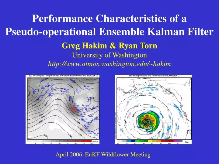
Performance Characteristics of a Pseudo-operational Ensemble Kalman Filter. Greg Hakim & Ryan Torn University of Washington http://www.atmos.washington.edu/~hakim. April 2006, EnKF Wildflower Meeting. Outline. Issues for limited-area EnKFs. Boundary conditions. Nesting.

E N D
Performance Characteristics of a Pseudo-operational Ensemble Kalman Filter Greg Hakim & Ryan Torn University of Washington http://www.atmos.washington.edu/~hakim April 2006, EnKF Wildflower Meeting
Outline • Issues for limited-area EnKFs. • Boundary conditions. • Nesting. • [Multiscale prior covariance.] • UW pseudo-operational system. • Performance characteristics. • Analysis of Record (AOR) test. • Experiments using the UW RT data. • Sensitivity & targeting. • Observation impact & thinning.
Boundary Conditions • Obvious choice: global ensemble, but… • Often ensembles too small. • Undesirable ensemble population techniques. • Different resolution, grids, etc. • Flexible alternatives (Torn et al. 2006). • Mean + random draws from N(0,B). • Mean + scaled random draws from climatology. • “error boundary layer” shallow due to obs.
1 2 Nesting • Grid 1: global ensemble BCs. • E.g. draws from N(0,B) or similar. • Grid 2: ensemble BCs from grid 1. • One-way nesting: straightforward. • Cycle on grid 1, then on grid 2. • Two-way: many choices; little experience. • Note: Hxb different on grids 1 and 2. • Issues at grid boundaries.
The Multiscale Problem • Sampling error • noise in obs est & prior covariance. • Ad hoc remedies • “localization” • Confidence intervals. • Multiscale problem. • Noise on smallest scales may dominate. • Need for scale-selective update?
Objectives of System • Evaluate EnKF in a region of sparse in-situ observations and complex topography. • Estimate analysis & forecast error. • Sensitivity: targeting & thinning.
Model Specifics • WRF Model, 45 km resolution, 33 vertical levels • 90 ensemble members • 6 hour analysis cycle • ensemble forecasts to t+24 hrs at 00 and 12 UTC • perturbed boundaries using fixed covariance perturbations from WRF 3D-VAR
Probabilistic Analyses 500 hPa height sea-level pressure Large uncertainty associated with shortwave approaching in NW flow
Microphysical Analyses 20 February 2005, 00 UTC model analysis composite radar
Ensemble Forecasts Analysis 24-hour forecast
Temperature Verification 12 hour forecast 24 hour forecast UW EnKFGFSCMCUKMO NOGAPS ECMWF
U-Wind Verification 12 hour forecast 24 hour forecast UW EnKFGFSCMCUKMO NOGAPS ECMWF
Moisture Verification (Td) 12 hour forecast 24 hour forecast UW EnKFGFSCMCUKMO NOGAPS ECMWF
No Assimilation Verification Winds Temperature UW EnKFNo Observations Assimilated
Analysis of Record Hourly surface analyses. EnKF covariances. Available t+30 minutes. 15 km resolution.
Sensitivity Analysis • Basic premise: • how do forecasts respond to changes in initial & boundary conditions, & the model? • Applications: • “targeted observations” & network design. • “targeted state estimation” (thinning). • basic dynamics research.
Adjoint approach Given J, a scalar forecast metric, one can show that: adjoint of resolvant • Need to run an adjoint model backward in time. • Complex code & lots of approximations • Does not account for state estimation or errors.
Ensemble Approach • Adjoint sensitivity weighted by initial-time error covariance. • Can evaluate rapidly without an adjoint model! • Can show: this gives response in J, including state estimation. With Brian Ancell (UW)
Sensitivity from the UW Real-time system Case study removing one observation. Metric: average MSL pressure over western WA
Sensitivity Demonstration How would a forecast change if buoy 46036 were removed?
12 UTC 5 Feb Sensitivity Sea-level pressure 850 hPa temperature
12 UTC 5 Feb. Analysis Change Analysis Change Forecast Sensitivity
Forecast Differences • Assimilating the surface pressure observation at buoy 46036 leads to a stronger cyclone. • Predicted Response: 0.63 hPa • Actual Response: 0.60 hPa
Observation Impact Adaptively sampling the obs datastream Thin by assimilating only high-impact obs.
Summary • BCs: flexibility & weak influence. • UW real-time system ~gov. center quality. • Moisture field better than most. • Surface AOR ~10 km. • Sensitivity analysis. • Ensemble targeting easy & flexible. • Adaptive DA (“thinning”).
AOR Opportunities “No propagate” update nested high resolution single member. assimilate using coarse-grid stats. can be done “now.” Deterministic propagation as above, but evolve high-res state. Full filter evolve & assimilate entire ensemble. 4DVAR with EnKF statistics. at least 3--5 years out.
AOR Challenges • True multiscale conditions (<15 km). • Scale-dependent sampling errors? • Bias estimation and removal. • EnKF allows state-dependent bias estimation. • Model errorestimation & removal. • Parameter estimation; model calibration. • Satellite radiance assimilation. • Kalman smoothing.
Observation Densities aircraft obs. cloud winds
Ensemble inliers/outliers inlier outlier