Download
1 / 55
550 likes | 766 Views
Being Normal. a.k.a. For Whom the Bell Tolls . FIRST QUIZ NEXT WEEK. BUSY DAY - DON’T BE LATE – LOTS TO DO. Multiple Choice. 40 questions. Lectures 1, 2, and 3. 10% of your course grade. In this room. 45 minutes. 8:10 start. 8:55 end. DO NOT MISS IT. THERE WILL BE NO MAKE-UPS.

E N D
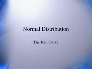
Being Normal a.k.a. For Whom the Bell Tolls
FIRST QUIZ NEXT WEEK BUSY DAY - DON’T BE LATE – LOTS TO DO. Multiple Choice. 40 questions. Lectures 1, 2, and 3. 10% of your course grade. In this room. 45 minutes. 8:10 start. 8:55 end. DO NOT MISS IT. THERE WILL BE NO MAKE-UPS.
To Do To Day Not the hardest stuff in stats but up there – it’s going to be a four day. Topics Curve(s) are good. Skewness and Kurtosis stats. z Scores. 4 Curve Pizza.
Curve(s) are Good A data based (almost) normal curve from a sample gives us an approximation of the mean and standard deviation for a population. No theory here – it’s all ABOUT THE data!
Curve(s) are Good The theoretical alwaysnormal curve is called normal because it is built on a set of known mathematical characteristics called “parameters”. These are mean and the standard deviation. No Data here – it’s all ABOUT THE THEORY!
Curve(s) are Good Because… If the curve of the population variable we are examining is almost normal, and… If the curve of the sample data we collect is almost normal, and… If we know the mathematical parameters of the perfect theoretical (non-data) curve, then… We can measure how far off the sample parameters will be from the population parameters, because… We can compare the perfect theoretical normal curve’s knownmathematical parameters to the sample curve’s actualdata-based parameters.
Curve(s) are Good Because… So what are the theoretical normal curves parameters? The mathematical arithmetic mean. The mathematical standard deviation. Because these tell us where any value willfall under the curve. And what are the normal sample curve’s parameters? The sample data’s arithmetic mean. The sample data’s standard deviation. Because these tell us where any sample value does fall under the curve.
Basic Characteristics of the Theoretical Normal Curve Data values are symmetrical about the mean 50% of all values 50% of all values Points of inflection Together these characteristics are called homoscedasticity, and the normal curve is said to be homoscedastic. Points of deflection Left tail Curve is asymptotic (never touches the x axis) Right tail Small or negative values Large or positive values Mean Median Mode all equal
IMPORTANT STUFF! IMPORTANT STUFF! IMPORTANT STUFF! Distribution Of Data Values Under The Normal Curve 50% of all values 50% of all values Areas under the curve are measured by the standard deviation. How to read: 34.13% of values fall between the mean and ±1s 13.59% of values fall between ±1s and ±2s of the mean 2.15% of values fall between ±2s and ±3s of the mean 0.13% of values are ±3s or more than the mean 34.13% 34.13% 2.15% 2.15% 13.59% 13.59% 0.13% 0.13% -3s -1s +1s +3s -2s +2s Mean IMPORTANT! Theoretical strength of normal curve is based on the proportions of values that MUST fall within specific distances from the means…
Distribution Of Data Values Under The Normal Curve 50% of all values 50% of all values 47.42% (13.59+34.13) 81.85% (34.13+34.13+13.59) 95.44% (13.59+34.13+34.13+13.59) 34.13% 34.13% 2.15% 2.15% 13.59% 13.59% 0.13% 0.13% +3s -1s -3s +1s -2s +2s Mean Any proportion of values can be calculated from these theoretical distributions
Significance Of Data Values Under The Normal Curve 50% of all values 50% of all values 34.13% 34.13% 2.15% 2.15% 13.59% 13.59% 0.13% 0.13% +1s +3s -2s -1s +2s -3s Mean Because of the distribution it follows that only 4.3% (2.15%+2.15%+0.13%+0.13%) of values in any dataset will lie 2 or more standard deviations from the mean and only 0.26% (0.13%+0.13%) will lie 3 or more standard deviations from the mean
Significance Of Data Values Under The Normal Curve 50% of all values 50% of all values 95% of data values 99% of data values 34.13% 34.13% 2.15% 2.15% 13.59% 13.59% 0.13% 0.13% Mean -2s +1s +2s +3s -1s -3s In fact 95% of data values will fall within 1.96 s and 99% within 2.58 sleaving us 95% or 99% sure that any value that exceeds these parameters is ‘significantly’ different than the mean.
The Magic Numbers In statistics confidence in your findings is expressed by confidence limits. Because we wish to be as sure as we can and still get a result we are very conservative in stating these limits. Acceptable confidence limits are never less than: 95% or 99% or higher depending on the problem being explored. THEREFORE, THE MAGIC NUMBERS ARE:
The Magic Numbers THEREFORE, THE MAGIC NUMBERS ARE: When a data value falls ± 1.96s from the mean we can be 95% sure it is significantly different than the mean. That is higher (+) than the mean or lower (-) than the mean. When a data value falls ± 2.58sfrom the mean we can be 99%sure it is significantly different than the mean. That is higher (+) than the mean or lower (-) than the mean.
Theorems From these theoretical considerations come two of the most important theorems in statistics. The first, Chebyshev’s theorem, deals with the proportional areas under the normal curve in terms of standard deviations. The second, the Central Limits Theorem (CLT), deals more directly with why we can trust our sample (because of the sampling distribution) and we will deal with these at the end of the course.
Theorem #1 Chebyshev’s Theorem: With normal distributions, a specific but decreasing proportion of all values will fall within kstandard deviations of the mean as kincreases That is: ±1s= 34.13% (@68%) of all data values ±2s= 13.59% (@27%) of all data values ±3s= 2.15 (4%) of all data values >3s= 0.13% (@0.3%) of all data values
Theorem #2 The Central Limits Theorem: If a sample size is large enough we can with measurable certainty say that thesampling distributionwill approximate a normal distribution. And what is a sampling distribution? Stay tuned until the exciting conclusion of this course to find out!
Other Types Of Curve Possible – Student’s ‘T’ Data values are symmetrical about the mean 50% of all values 50% of all values Points of inflection Points of deflection Left tail Right tail Mean Median Mode all equal Small or negative values Large or positive values Student’s ‘t’ curve for small samples has a larger proportion of values in the tails, otherwise characteristics are the same
Other Types of Curve Possible Chi Square Data values are not distributed symmetrically about the mean Left tail Right tail Small or negative values Large or positive values Mean Median Mode differ Mean Median Mode all equal Chi square curve is skewed with disproportionate share of values in each tail
Other Types of Curve Possible F Distributions
Summing up the Normal Curve The normal curve from theoryis not based on data but on mathematics. It allows us to calculate the proportion of data values falling under different areas of the curve. “Real world” data distributions (especially samples) that approximate normal distributions make the theoretical principles of the normal curve useful to us. Why?
Summing up the Normal Curve Because we can be 95% sure that any data values that fall beyond ±1.96s of the mean are significantly different than the mean (and hence most other values). This is a good thing because without the theoretical curve we could not do inferential statistics on the “real world” data we collect. Again the usefulness of the mean and standard deviation are evident.
Summing up the Normal Curve The usefulness of the mean and the standard deviation should be clear. It should also be clear that if the distribution is not normal then the proportions will not meet the parametersof the normal distribution. That is, the 1.96s for 95% and the 2.58s for the 99%. Thus, any dataset that does not meet the normality criteria will not be robustand neither will be the parametric statistics you use.
Normality By The Numbers: Skewness and Kurtosis Statistics
Interpreting Frequency DistributionsSkewness (Lean) Sample A Positively skewed (tail goes right) Sample B Not skewed (tails equal) Sample C Negatively skewed (tail goes left) Only sample B is normally distributed. F Median Median Mode Median Mode Mode
Interpreting Frequency DistributionsSkewness Statistic Where: Skis Pearson’s measure of skewness is the mean mis the median s is the standard deviation
Interpreting the Skewness Statistic No skewness? Sk = 0 Skewed positive or tail to high values/right? Sk = positive # Skewed negative or tail to low values/left? Sk = negative # But how negative or positive do the numbers have to be for the distribution to be considered skewed? That’s where the standard error of skewnessstatistic come in handy…
Interpreting the Skewness StatisticThe Standard Error of Skewness Where: ses is the standard error of skewness value nis the number of cases in your dataset Interpretation: When your skewness statistic (Sk) is equal to or greater than 2 *ses you have significant negative or positive skewness to your data. THAT IS, THE DISTRIBUTION IS NON-NORMAL.
Interpreting the Skewness StatisticThe Standard Error of Skewness Example: GNI per capita of 163 nations = +1.61 skewness ses = √(6/163) = √.0368 = 0.192 ses*2 = 0.192*2 = 0.384 Since +1.61 is much higher than 0.384 we can say that the global distribution of incomes has a significant positive skewness – that is, more lower than higher incomes. This is a result you would have expected given that there are far more poor nations than rich nations. NOTE: When calculating the ses, the ‘sign’ on the skewness statistic does not matter – it tells you direction only.
Interpreting Frequency DistributionsKurtosis Sample A Leptokurtic Small standard deviation Sample B No kurtosis Normal standard deviation Only Sample B Is normal F Sample C Platykurtic Large standard deviation
Interpreting Frequency DistributionsKurtosis Statistic Whoa!!! Gotta get the tee shirt! Where: K is kurtosis x is a value in the dataset is the mean n is the number of data values in the dataset s is the standard deviation
Interpreting the Kurtosis Statistic No kurtosis? K = 0 Negative kurtosis (platykurtic or flat)? K = negative # Positive kurtosis (leptokurtic or peaked)? K = positive # But how negative or positive do the numbers have to be for the distribution to be considered kurtotic? That’s where the standard error of kurtosis statistic come in handy…
Interpreting the Kurtosis StatisticThe Standard Error of Kurtosis Where: sek is the standard error of kurtosis value n is the number of cases in your dataset Interpretation: When your kurtosis statistic (K) is equal to or greater than 2 *sekyou have significant negative or positive kurtosis to your data. THAT IS, THE DISTRIBUTION IS NON-NORMAL.
Interpreting the Kurtosis StatisticThe Standard Error of Kurtosis Example: GNI per capita of 163 nations = +2.42 kurtosis sek= √(24/163) = √0.147 = 0.383 and therefore sek*2 = 0.383 * 2 = +0.766 Since +2.42 is much higher than 0.766 we can say that the global distribution of incomes has a significant positive or peaked kurtosis – that is, more lower than higher incomes clustered around the median This is a result you would have expected given that there are far more poor nations than rich nations. NOTE: When calculating the sek, the ‘sign’ on the kurtosis statistic does not matter – it tells you direction only.
The Standard Normal Curve Normal distributions can be transformed into another useful distribution called the standard normal curve, which has a mean of 0 and a standard deviation of 1. By calculating a statistic called the zscore for data values in a dataset you are able to replace all data values with a number that indicates how many standard deviations the value lies from the mean. This allows you to: • compare different datasets; (2) flag significantly different values (values that fall in the tails of the distribution).
The zScore Where: zis the z score xis the individual data value is the arithmetic mean of the data s is the standard deviation of the data Each data value will get a corresponding ± zscore that indicates how many standard deviations it is away from the mean and in what direction (that is, is it larger (+) or smaller (-) than the mean) and by how much.
Interpreting the z score The z score is the number of standard deviations above (+) or below (-) the mean that a particular data value (x) lies. Thus… We can tell if the data value (x) lies in the tails of the data’s distribution, and if so which one. How?... Using the characteristics of the normal curve we know the proportion of values within specific numbers of standard deviations from the mean. Hence z scores greater than ±1.96 or ± 2.58 tell you that you can be 95% or 99% sure the associated value is significantly different than the mean of all the other data values in the distribution (dataset). WHY?
Theorem #1This is Why: Chebyshev’s Theorem: With normal distributions, a specific but decreasing proportion of all values will fall within k standard deviations of the mean as k increases That is: ±1s= 34.13% (@68%) of all data values ±2s= 13.59% (@27%) of all data values ±3s= 2.15 (4%) of all data values >3s= 0.13% (@0.3%) of all data values
A z Score Example Your grade in Stats = 80% Your grade in Economics = 90% In which course did you do the best? Most would say economics, including Ryerson when they calculate your grade! But are they correct? If the variability across the grades is low, then getting an 80% in stats might be much more difficult than getting a 90% in economics. So let’s see.
All is not what it appears…. The real question about how well you did is not what grade you got but how many other students did you beat to get it. Given the data above we can calculate that your grade in stats was 3sabove the mean and your grade in economics was only 2sabove the mean.
All is not what it appears…. Using the normal curve you know that in stats you had to beat 99.87% of the other students to get your grade, but in economics you ‘only’ had to beat 97.85% of them. Clearly you beat a tougher crowd in stats than in economics.
Decision making… Ponder this: Would you like your Ryerson grade to be measured as a zscore or as a grade out of 100%? (P.S. This procedure works in both directions )
zScore Example Comparing the z scores tells you how each data value relates to the mean and sof its dataset in the same terms. E.G. 44 = 0.87 sabove its mean 3.1 = 1.89 sabove its mean. Comparing the data values or the means and sof these two datasets does not tell you anything.
The z score and significant results A z score redefines a value in terms of standard deviations for the dataset to which the value belongs Therefore it can be used to estimate if a value is significantly different than other values in its dataset This is much more useful than the starting value, which can be misleading when compared to other values (e.g. grades example) This uses the 1.96s and 2.58s rule: 1.96=95% or 1 chance in 20 of occurring 2.58=99% or 1 chance in 100 of occurring Once again Chebyshev rules!
Summing Up the z Score The z score provides a single number that allows you to compare very different data values. The arithmetic mean of a set of z scores is always zero and the standard deviation always 1. Negative z score values indicate that the associated data value is below the mean and positive z scores tell you that it is above the mean. Any dataset value that is the same as the mean for the dataset will have a z score of 0 A z score of 1.96 has five chances in a hundred of occurring, while a z score of 2.58 has one chance in a hundred of occurring.
Distributions or ‘Curves’ The most important concept in statistics. If you understand what these four basic curves are and how they relate to one another, you will understand how statistics works.
The Various ‘Normal’ Distributions in Summary THE POPULATION DISTRIBUTION OR CURVE This ‘curve’ is based on the population’s assumed data distribution. Many social science and science variables turn out to be ‘normally distributed’ – more or less representing a bell curve. Therefore any sample taken properly from them will show approximately the same curve.