Download
1 / 86
860 likes | 947 Views
Design of Experiment and Assessing Interactions within Atmospheric Processes. Dev Niyogi North Carolina State University Email: dev_niyogi@ncsu.edu. Human thinking is logical , sequential, and linear Real world is Convulated, Non-linear, and Interactive. Some References.

E N D
Design of Experiment and Assessing Interactions within Atmospheric Processes Dev Niyogi North Carolina State University Email: dev_niyogi@ncsu.edu
Human thinking islogical , sequential, and linearReal world isConvulated, Non-linear, and Interactive
Some References • Mesoscale Meteorological Modeling, Roger Pielke Sr., Second Edition. (blue.atmos.colostate.edu) • Box, Hunter and Hunter, Design of Experiment, 1987 • Stein and Alpert, Factor Separation Analysis, J. Atmos. Sci. 1993 • Alpert et al., How good are sensitivity studies?, J. Atmos. Sci. 1995 • Henderson- Sellers, A fractional – factorial approach, J. Climate, 1993 • Niyogi et al. 1995, Env. Mod. Assess, Statistical – Dynamical Experiments • Niyogi et al. 1999 Uncertainty in initial specification- hierarchy; Boun. Layer Meteorol. • Niyogi et al. 2002 Land surface response- midlatitudes and tropics, J. Hydromet (www4.ncsu.edu/~dsniyogi)
Sensitivity Analysis • Inherent component of model studies • Both observational as well as numerical modeling studies rely on sensitivity analysis • Approach – Change a variable see the effect on the outcome
Sensitivity Analysis • Objective • Understand the cause – effect relationship • Understand the relative importance of the different processes affecting the outcome • Develop focused efforts on improving input for critical variables (GIGO) • Develop if – then scenarios for policy makers; socioeconomic analyses, … • Evaluate models • …
OAT Analysis • Inherent component of model studies • Both observational as well as numerical modeling studies rely on sensitivity analysis • Approach – Change a variable see the effect on the outcome
Summary of OAT Analysis - Linear results • Interactions need to be extracted in a ad-hoc manner / subjectively • Results state ‘what is happening’ and not ‘how it is happening’ in the analysis
Sensitivity Analysis using Observations • Needs careful planning (several known and unknown feedbacks possible) • Effects cannot be “switched off” reliably (unlike in a model) • Modeling OAT sensitivities could be used for developing trends and extrapolations • Observational OAT can be largely used for hypothesis tests (too many factors; too much noise) • KISS (Keep it Simple Stupid) syndrome can be boon and a bane (too much confounding and original results may be lost)
Sensitivity Analysis using Observations • Either Absent / Present scenarios tested • Cloud cover and no clouds; • Irrigation and no irrigation • Fertilizer and no fertilizer • Or High / Low scenarios tested • High soil moisture and low soil moisture • Ambient CO2 and Doubled CO2
High soil moisture Low Soil Moisture LESS DIFFUSE Measure the environment below the two experimental domains and evaluate the outcome (temperature, crop yield, photosynthesis, …)
Ambient versus doubled CO2 levels Measure the environment below the two experimental domains and evaluate the outcome (temperature, crop yield, photosynthesis, …)
Example of a field sensitivity study Field Measurements at NCSU to assess diffuse radiation feedback Does increase in diffuse radiation fraction help crop yield?
MORE DIFFUSE LESS DIFFUSE Measure the environment below the two experimental domains and evaluate the outcome (temperature, crop yield, photosynthesis, …)
Comparison of OAT in models and in field • Models – High Diffuse - > more photosynthesis • Observations – High diffuse -> less temperatures -> more shade on crops -> leaf geometry changes -> large fluctuations
Clustering and Cleaning eventually gets the right results from observations ;always an element of uncertainty that results could have gone ‘other way’ too in some scenarios. Q: Should the observations be relied on for testing models? (of course yes; but don’t use observations as the truth!)
Diffuse radiation effect under cloudy conditions Diffuse radiation effect under non-cloudy conditions
Clustering and Synthesis of Sensitivity Experimentation Data Interpretation High LAI case Observations and Models need to go hand in hand to help develop the understand (don’t treat observations alone as the truth) Low LAI case
Too many model evaluation studies; particularly for synthesizing processes rely overtly on observations; Observations are essential for model testing and evaluation But observations are also chaotic QUESTION OBSERVATIONS Know the uncertainty associated with the measurements Models need not agree with all observations to be good Models give time dependent ensemble output; observations at a given time are just that- observation at that point and/or time Even observations have feedbacks embedded which have not been traditionally extracted
No I am not a modeler! Models do not represent the reality but neither do observations unless they are clearly synthesized. Need to synthesize results (observations and model output) in a nonlinear / feedback and interaction perspective
Feedbacks and Interactions • Feedback processes are a result of cause and effect. • That is, one follows the other in a time sequential manner • The processes could be coupled as well as uncoupled • A -> B -> C • A-> B -> C ->a -> b -> c …
Feedbacks and Interactions • Interactions, on the other hand, implies concurrence. • There is no cause and effect associated with the interactions and a simultaneous effect is associated. • A -> B -> C and D
Interactions • Examples • Medicine and Prescription Drug Use • Drug ‘A’ will lead to helping relieve headache • Drug ‘A’ taken while taking Drug ‘B’ will cause nausea • Drug ‘A’ taken with coffee can cause marked improvement • Nutrition and Health • Results show wine is good for health; add to your diet; • red wine is better; • true for people exercising • Same effect as grape juice • Wine is not necessary, take out of your diet • All are examples of real-life interactions occurring which need to be resolved
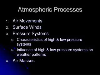
Feedbacks and Interactions • Surface Energy Balance & Evapotranspiration • Rn = Etr + Shf + storage; Etr = Eg+Tr • Gradients in Surface Fluxes • Non-classical Circulation • Convection and Cumulus Formation • Precipitation and Land Use Change • Regional Climate Change
Factor Separation (FacSep) Analysis (Stein and Alpert, 1993; Alpert et al. 1995; J. Atmos. Sci.)Interaction Explicit Analysis of effect of simultaneous soil moisture and CO2 changes on terrestrial feedback Eo = Fo = f [ CO2 - , Moist -] F1 = f [ CO2 + , Moist - ] F2 = f [CO2 - , Moist + ] F12 = f [ CO2 + , Moist + ] E(CO2) = F1 - Eo E(SM) = F2 - Eo E(CO2:SM) = F12 - (F1+F2) - Fo
FacSep results can be interpreted and analyzed using either time series tools or other traditional descriptive statistics routinely used in One at A Time Sensitivity Analysis
Feedbacks and Interactions • Full Factorial (2^n) I.e. 8 combns for 3 factors; 16 for 4; 32 for 5 etc. • At three settings (low, medium, and high) this will be 3^n I.e. 27 for 3 factors, 64 for 4 factors etc. • Solution? • Fractional Factorial Approach (statistical design) • Some confounding (all interactions / combinations not resolved) • Several design matrices routinely available (statistics texts, software packages, internet, …)
Fractional Factorial Designs • “Resolution 5” all main effects and two-factor interactions resolved (FF0516) • “Resolution 4” some two factor Xns retained (FF0616) • “Resolution 3” Screening type; interactions may not be resolved (FF0508) • Nonlinear response surface (fc0318) • Effect = Main Effect + Interaction • Main effect plots -> Pareto plot -> Interaction plots-> normal plots / active contrast / gambler plots -> diagnosis of feedbacks and interactions
Summary of OAT Analysis - Linear results • Interactions need to be extracted in a ad-hoc manner / subjectively • Results state ‘what is happening’ and not ‘how it is happening’ in the analysis