Download
1 / 135
1.37k likes | 1.6k Views
Datalog and Emerging Applications: an Interactive Tutorial . Shan Shan Huang T.J . Green Boon Thau Loo. SIGMOD 2011 Athens, Greece June 14, 2011. A Brief History of Datalog. Declarative networking. C ontrol + data flow. BDDBDDB. SecureBlox. Orchestra CDSS.

E N D
Datalog and Emerging Applications: an Interactive Tutorial Shan ShanHuang T.J. Green Boon ThauLoo SIGMOD 2011 Athens, Greece June 14, 2011
A Brief History of Datalog Declarative networking Control + data flow BDDBDDB SecureBlox Orchestra CDSS Workshop on Logic and Databases Data integration Information Extraction Hey wait… there ARE applications! No practical applications of recursive query theory … have been found to date. -- Hellerstein and Stonebraker “Readings in Database Systems” ‘77 ‘95 ‘05 ‘07 ‘08 ’80s … ‘02 ‘10 Doop (pointer-analysis) Access control (Binder) LDL, NAIL, Coral, ... Evita Raced .QL
Today’s Tutorial, or,Datalog: Taste it Again for the First Time • We review the basics and examine several of these recent applications • Theme #1: lots of compelling applications, if we look beyond payroll / bill-of-materials / ... • Some of the most interesting work coming from outside databases community! • Theme #2: language extensions usually needed • To go from a toy language to something really usable
(Asynchronously!) An Interactive Tutorial ^ • INSTALL_LB : installation guide • README : structure of distribution files • Quick-Start guide : usage • *.logic : Datalog examples • *.lb : LogicBlox interactive shell script (to drive the Datalog examples) • Shan Shan and other LogicBlox folks will be available immediately after talk for the “synchronous” version of tutorial
Outline of Tutorial June 14, 2011: The Second Coming of Datalog! • Refresher: Datalog 101 • Application #1: Data Integration and Exchange • Application #2: Program Analysis • Application #3: Declarative Networking • Conclusions
Datalog Refresher: Syntax of Rules Datalog rule syntax: <result> <condition1>, <condition2>, … , <conditionN>. Head Body • Body consists of one or more conditions (input tables) • Head is an output table • Recursive rules: result of head in rule body
Example: All-Pairs Reachability R1: reachable(S,D)<-link(S,D). R2: reachable(S,D)<-link(S,Z),reachable(Z,D). “For all nodes S,D, If there is a link from S to D, then S can reach D”. link(a,b) – “there is a link from node a to node b” reachable(a,b) – “node a can reach node b” Input: link(source, destination) Output: reachable(source, destination)
Example: All-Pairs Reachability R1: reachable(S,D)<-link(S,D). R2: reachable(S,D)<-link(S,Z),reachable(Z,D). “For all nodes S,D and Z, If there is a link from S to Z, AND Z can reach D, then S can reach D”. Input: link(source, destination) Output: reachable(source, destination)
Terminology and Convention • An atomis a predicate, or relation name with arguments. • Convention: Variables begin with a capital, predicates begin with lower-case. • The head is an atom; the body is the AND of one or more atoms. • Extensional database predicates (EDB) – source tables • Intensional database predicates (IDB) – derived tables reachable(S,D)<- link(S,Z),reachable(Z,D) .
Negated Atoms Not “cut” in Prolog. • We may put ! (NOT) in front of a atom, to negate its meaning. • Example: For any given node S, return all nodes D that are two hops away, where D is not an immediate neighbor of S. • twoHop(S,D) • <- link(S,Z), • link(Z,D) • ! link(S,D). link(S,Z) link(Z,D) Z D S
Safe Rules • Safety condition: • Every variable in the rule must occur in a positive (non-negated) relational atom in the rule body. • Ensures that the results of programs are finite, and that their results depend only on the actual contents of the database. • Examples of unsafe rules: • s(X) <- r(Y). • s(X) <- r(Y), ! r(X).
Semantics • Model-theoretic • Most “declarative”. Based on model-theoretic semantics of first order logic. View rules as logical constraints. • Given input DB I and Datalog program P, find the smallest possible DB instance I’ that extends I and satisfies all constraints in P. • Fixpoint-theoretic • Most “operational”. Based on the immediate consequence operator for a Datalog program. • Least fixpoint is reached after finitely many iterations of the immediate consequence operator. • Basis for practical, bottom-up evaluation strategy. • Proof-theoretic • Set of provable facts obtained from Datalog program given input DB. • Proof of given facts (typically, top-down Prolog style reasoning)
The “Naïve” Evaluation Algorithm Start: IDB = 0 • Start by assuming all IDB relations are empty. • Repeatedly evaluate the rules using the EDB and the previous IDB, to get a new IDB. • End when no change to IDB. Apply rules to IDB, EDB yes Change to IDB? no done
Naïve Evaluation reachable link reachable(S,D) <- link(S,D). reachable(S,D) <- link(S,Z), reachable(Z,D).
Semi-naïve Evaluation • Since the EDB never changes, on each round we only get new IDB tuples if we use at least one IDB tuple that was obtained on the previous round. • Saves work; lets us avoid rediscovering most known facts. • A fact could still be derived in a second way.
Semi-naïve Evaluation reachable link reachable(S,D) <- link(S,D). reachable(S,D) <- link(S,Z), reachable(Z,D).
Recursion with Negation Example: to compute all pairs of disconnected nodes in a graph. reachable(S,D) <- link(S,D). reachable(S,D) <- link(S,Z), reachable(Z,D). unreachable(S,D) <- node(S), node(D), ! reachable(S,D). unreachable Stratum 1 • Precedence graph : • Nodes = IDB predicates. • Edge q <- p if predicate q depends on p. • Label this arc “–” if the predicate p is negated. -- reachable Stratum 0
Stratified Negation unreachable Stratum 1 reachable(S,D) <- link(S,D). reachable(S,D) <- link(S,Z), reachable(Z,D). unreachable(S,D) <- node(S), node(D), ! reachable(S,D). -- reachable Stratum 0 • Straightforward syntactic restriction. • When the Datalog program is stratified, we can evaluate • IDB predicates lowest-stratum-first. • Once evaluated, treat it as EDB for higher strata. • Non-stratified example: p(X) <- q(X), ! p(X).
A Sneak Preview… • Data integration • Skolem functions • Program analysis • Type-based optimization • Declarative networking • Aggregates, aggregate selections • Incremental view maintenance • Magic sets
Suggested Readings • Survey papers: • A Survey of Research on Deductive Database Systems, Ramakrishnan and Ullman, Journal of Logic Programming, 1993 • What you always wanted to know about datalog (and never dared to ask), by Ceri, Gottlob, and Tanca. • An Amateur’s Expert’s Guide to Recursive Query Processing, Bancilhon and Ramakrishnan, SIGMOD Record. • Database Encyclopedia entry on “DATALOG”. GrigorisKarvounarakis. • Textbooks: • Foundations in Databases. Abiteboul, Hull, Vianu. • Database Management Systems, Ramakrishnan and Gehkre. Chapter on “Deductive Databases”. • Acknowledgements: • Jeff Ullman’s CIS 145 class lecture slides. • RaghuRamakrishnan and Johannes Gehrke’s lecture slides for Database Management Systems textbook.
Outline of Tutorial June 14, 2011: The Second Coming of Datalog! • Refresher: Datalog 101 • Application #1: Data Integration and Exchange • Application #2: Program Analysis • Application #3: Declarative Networking • Conclusions
Datalog for Data Integration • Motivation and problem setting • Two basic approaches: • virtual data integration • materialized data exchange • Schema mappings and Datalog with Skolem functions
The Data Integration Problem • Have a collection of related data sources with • different schemas • different data models (relational, XML, plain text, ...) • different attribute domains • different capabilities / availability • Need to cobble them together and provide a uniform interface • Want to keep track of what came from where • Focus here: solving problem of different schemas (schema heterogeneity) for relational data
Mediator-Based Data Integration Basic idea: use a globalmediated schema to provide a uniform query interface for the heterogeneous data sources . Global mediated schema ? ? ? ? Source schemas Local data sources
Mediator-Based Virtual Data Integration Integrated query results Query over global schema Query may be recursive Global mediated schema Query results Declarative schema mappings Reformulated query over local schemas Source schemas Local data sources Reformulation may be (necessarily) recursive
Materialized Data Exchange Declarative schema mappings Query results Query Mappings may be recursive Materialized mediated (target) database Global mediated schema (aka target schema) Declarative schema mappings Data exchange step (construct mediated DB) Source schema(s) Local data source(s)
Peer-to-Peer Data Integration (Virtual or Materialized) Results Query Peer A Peer E Peer C Recursion arises naturally as peers add mappings to each other Query Results Peer B Peer D
How to Specify Mappings? • Many flavors of mapping specifications: LAV, GAV, GLAV, P2P, “sound” versus “exact”, ... • Unifying formalism: integrity constraints • different flavors of specifications correspond to different classes of integrity constraints • We focus on mappings specified using tuple-generating dependencies (a kind of integrity constraint) • These capture (sound) LAV and GAV as special cases, and much of GLAV and P2P as well • and, close relationship with Datalog!
Logical Schema Mappings viaTuple-Generating Dependencies (tgds) • A tuple-generating dependency (tgd) is a first-order constraint of the form where ϕ and ψ are conjunctions of relational atoms For example: “The name and address of every employee should also be recorded in the name and address tables, indexed by ssn.” ∀X ϕ(X) → ∃Yψ(X,Y) ∀ Eid, Name, Addr employee(Eid, Name, Addr) → ∃ Ssn name(Ssn, Name) ∧address(Ssn, Addr)
What Answers Should Queries Return? • Challenge: constraints leave problem “under-defined”: for given local source instance, many possible mediated instances may satisfy the constraints. ∀ Eid, Name, Addr employee(Eid, Name, Addr) → ∃ Ssn name(Ssn, Name) ∧address(Ssn, Addr) CONSTRAINT: LOCAL SOURCE MEDIATED DB #2 MEDIATED DB #1 ...ETC... employee name name ... address address What answers should q return? ... Which mediated DB should be materialized? QUERY: q(Name) <- name(Ssn, Name), address(Ssn, _).
Certain Answers Semantics Basic idea: query should return those answers that would be present for any mediated DB instance (satisfying the constraints). MEDIATED DB #1 LOCAL SOURCE MEDIATED DB #2 ...ETC... employee name name ... address address QUERY: ... q(Name) <- name(Ssn, Name), address(Ssn, _). q q certain answers to q ... ∩ ∩ =
Computing the Certain Answers • A number of methods have been developed • Bucket algorithm [Levy+ 1996] • Minicon [Pottinger & Halevy 2000] • Inverse rules method [Duschka & Genesereth 1997] • ... • We focus on the Datalog-based inverse rules method • Same method works for both virtual data integration, and materialized data exchange • Assuming constraints are given by tgds
Inverse Rules: Computing Certain Answers with Datalog • Basic idea: a tgd looks a lot like a Datalog rule (or rules) • So just interpret tgds as Datalog rules! (“Inverse” rules.) Can use these to compute the certain answers. • Why called “inverse” rules? In work on LAV data integration, constraints written in the other direction, with sources thought of as views over the (hypothetical) mediated database instance The catch: what to do about existentially quantified variables... ∀ X, Y, Z foo(X,Y) ∧ bar(X,Z) → biz(Y,Z) ∧ baz(Z) tgd: • biz(X,Y,Z) <- foo(X,Y), bar(X,Z). • baz(Z) <- foo(X,Y), bar(X,Z). Datalog rules:
Inverse Rules: Computing Certain Answers with Datalog (2) • Challenge: existentially quantified variables in tgds • Key idea: use Skolem functions • think: “memoized value invention” (or “labeled nulls”) • Unlike SQL nulls, can join on Skolem values: ∀ Eid, Name, Addr employee(Eid, Name, Addr) → ∃ Ssn name(Ssn, Name) ∧address(Ssn, Addr) name(ssn(Name, Addr), Name) <- employee(_, Name, Addr). address(ssn(Name, Addr), Addr) <- employee(_, Name, Addr). ssn is a Skolem function query _(Name,Addr) <- name(Ssn,Name), address(Ssn,Addr).
Semantics of Skolem Functions in Datalog • Skolem functions interpreted “as themselves,” like constants (Herbrand interpretations): not to be confused with user-defined functions • e.g., can think of interpretation of term ssn(“Alice”, “1 Main St”) as just the string (or null labeled by the string) ssn(“Alice”, “1 Main St”) • Datalog programs with Skolem functions continue to have minimal models, which can be computed via, e.g., bottom-up seminaive evaluation • Can show that the certain answers are precisely the query answers that contain no Skolem terms. (We’ll revisit this shortly...) • But: the models may now be infinite!
Termination and Infinite Models • Problem: Skolem terms “invent” new values, which might be fed back in a loop to “invent” more new values, ad infinitum • e.g., “every manager has a manager” • Option 1: let ‘er rip and see what happens! (Coral, LB) • Option 2: use syntactic restrictions to ensure termination... manager manager(X) <- employee(_, X, _) . manager(m(X)) <- manager(X). employee m is a Skolem function
Ensuring Termination of Datalog Programs with Skolems via Weak Acyclicity vertex for each (predicate, index) • Draw graph for Datalog program as follows: (employee, 2) manager(X) <- employee(_, X, _) . manager(m(X)) <- manager(X). (employee, 1) (employee, 3) Cycle through dashed edge! Not weakly acyclic (manager, 1) variable occurs as arg #2 to employee in body, arg #1 to manager in head variable occurs as arg #1 to manager in body and as argument to Skolem (hence dashes) in arg #1 to manager in head • If graph contains no cycle through a dashed edge, then P is called weakly acyclic
Ensuring Termination via Weak Acyclicity (2) • Another example, this one weakly acyclic: (emp, 2) (emp, 3) (emp, 1) name(ssn(Name,Addr),Name) <- emp(_,Name,Addr). addr(ssn(Name,Addr),Addr) <- emp(_,Name,Addr). query _(Name,Addr) <- name(Ssn,Name), address(Ssn,Addr) ; _(Addr,Name). (addr, 1) (name, 1) (addr, 2) (name, 2) has cycle, but no cycle through dashed edge; weakly acyclic (_, 1) (_, 2) Theorem: bottom-up evaluation of weakly acyclic Datalog programs with Skolems terminates in # steps polynomial in size of source database.
Once Computation Stops, What Do We Have? ∀ Eid, Name, Addr employee(Eid, Name, Addr) → ∃ Ssn name(Ssn, Name) ∧address(Ssn, Addr) tgd: name(ssn(Name, Addr), Name) <- employee(_, Name, Addr). address(ssn(Name, Addr), Addr) <- employee(_, Name, Addr). datalog rules: MEDIATED DB #3 MEDIATED DB #2 MEDIATED DB #1 LOCAL SOURCE name name name employee ... address address address ... Among all the mediated DB instances satisfying the constraints (solutions), #2 above is universal: can be homomorphically embedded in any other solution.
Universal Solutions Are Just What is Needed to Compute the Certain Answers Proof (crux): use universality of materialized DB. • Theorem: can compute certain answers to Datalog program q over target/mediated schema by: • evaluating q on materialized mediated DB (computed using inverse rules); then • (2) crossing out rows containing Skolem terms.
Notes on Skolem Functions in Datalog • Notion of weak acyclicity introduced by Deutsch and Popa, as a way to ensure termination of the chase procedure for logical dependencies (but applies to Datalog too). • Crazy idea: what if we allow arbitrary use of Skolems, and forget about computing complete output idb’s bottom-up, but only partially enumerate their contents, on demand, using top-down evaluation? • And, while we’re at it, allow unsafe rules too? • This is actually a beautiful idea: it’s called logic programming • Skolem functions (aka “functor terms”) are how you build data structures like lists, trees, etc. in Prolog • Resulting language is Turing-complete
Summary: Datalog for Data Integration and Exchange • Datalog serves as very nice language for schema mappings, as needed in data integration, provided we extend it with Skolem functions • Can use Datalog to compute certain answers • Fancier kinds of schema mappings than tgds require further language extensions; e.g., Datalog +/- [Cali et al 09] • Can also extend Datalog to track various kinds of data provenance, very useful in data integration • Using semiring-based framework [Green+ 07]
Some Datalog-Based Data Integration/Exchange Systems • Information Manifold [Levy+ 96] • Virtual approach • No recursion • Clio [Miller+ 01] • Materialized approach • Skolem terms, no recursion, rich data model • Ships as part of IBM WebSphere • Orchestra CDSS [Ives+ 05] • Materialized approach • Skolem terms, recursion, provenance, updates
Datalog for Data Integration: Some Open Issues • Materialized data exchange: renewed need for efficient incremental view maintenance algorithms • Source databases are dynamic entities, need to propagate changes • Classical algorithm DRed [Gupta+ 93] often performs very badly; newer provenance-based algorithms [Green+ 07, Liu+ 08] faster but incur space overhead; can we do better? • Termination for Datalog with Skolems • Improvements on weak ayclicity for chase termination, translate to Datalog; more permissive conditions always useful! • Is termination even decidable? (Undecidable if we allow Skolems and unsafe rules, of course.)
Outline of Tutorial June 14, 2011: The Second Coming of Datalog! • Refresher: basics of Datalog • Application #1: Data Integration and Exchange • Application #2: Program Analysis • Application #3: Declarative Networking • Conclusion
Program Analysis • What is it? • Fundamental analysis aiding software development • Help make programs run fast, help you find bugs • Why in Datalog? • Declarative recursion • How does it work? • Really well! An order-of-magnitude faster than hand-tuned, Java tools • Datalog optimizations are crucial in achieving performance
Understanding Program Behavior testing (without actually running the program) what is animal? what is thing? animal.eat( (Food) thing); points-to analyses through what method does it eat?
Optimizations what is animal? it’s a Dog what is thing? it’s Chocolate animal.eat( (Food) thing); virtual call resolution type erasure through what method does it eat? class Dog { void eat(Food f) { … } }
Bug Finding what is animal? it’s a Dog what is thing? it’s Chocolate animal.eat( (Food) thing); ChokeExceptionnever caught = BUG Dog + Chocolate = BUG through what method does it eat? class Dog { void eat(Food f) { … } }