Download
1 / 6
60 likes | 172 Views
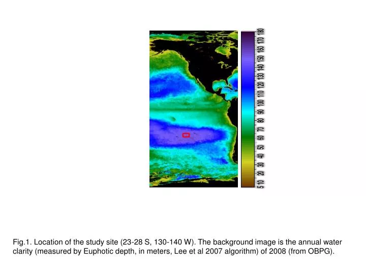
Fig.1. Location of the study site (23-28 S, 130-140 W). The background image is the annual water clarity (measured by Euphotic depth, in meters, Lee et al 2007 algorithm) of 2008 (from OBPG). Stations:. Rrs-derived a(420) [m -1 ]. 1:1. (a). a(420) [m -1 ]. Rrs-derived a ph (420) [m -1 ].

E N D
Fig.1. Location of the study site (23-28 S, 130-140 W). The background image is the annual water clarity (measured by Euphotic depth, in meters, Lee et al 2007 algorithm) of 2008 (from OBPG).
Stations: Rrs-derived a(420) [m-1] 1:1 (a) a(420) [m-1] Rrs-derived aph(420) [m-1] Rrs-derived adg(420) [m-1] 1:1 1:1 (b) (c) ag(420) [m-1] ap(420) [m-1] Fig.2. Comparison between remote-sensing inversions and values determined independently by other means, all at 420 nm. (a) total absorption; (b) particulate absorption; (c) gelbstoff absorption. Values for X-axis from Table 1 in Morel et al (2007).
aph(443) [m-1] adg(443) [m-1] (a) (b) Month-Year Month-Year Fig.3. Monthly times series of primary optical properties derived from SeaWiFS observations (1/1998 – 12/2007). (a): phytoplankton absorption coefficient (443 nm); (b) detritus/gelbstoff absorption coefficient (443 nm); (c) “particle” backscattering coefficient (555 nm). Overlaid on (a) and (b) are empirical models (open sysmbol) to highlight the seasonal and interannual dynamics. bbp(555) [m-1] (c) Month-Year
R2 = 0.423 R2 = 0.122 aph(443) [m-1] adg(443) [m-1] R2 = 0.042 R2 = 0.108 Month-Year Month-Year Fig.4. Internannual dynamics of the background and seasonal intensity of aph and adg.
R2 = 0.106 R2 = 0.629 adg(443) [m-1] aph(443) [m-1] SST [oC] SST [oC] Fig.5. Relationship between SST and aph (left), and between SST and adg (right) .
Chla [mg/m3] Chla [mg/m3] Month-Year Month-Year Fig.6. (a) Monthly time series of chlorophyll-a concentration derived from SeaWiFS. Blue symbol and line for Chla derived from the aph results, with the formula from Bricaud et al (2004): aph(443) = 0.0654 Chla0.728. (b) As Fig.3, background and intensity of Chla, with Chla from the empirical OC4 algorithm.