Download
1 / 73
770 likes | 908 Views
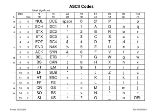
Digital Communication Systems Lecture-2, Prof. Dr. Habibullah Jamal. Under Graduate, Spring 2008. Formatting. Example 1: In ASCII alphabets, numbers, and symbols are encoded using a 7-bit code. A total of 2 7 = 128 different characters can be represented using

E N D
Digital Communication SystemsLecture-2, Prof. Dr. Habibullah Jamal Under Graduate, Spring 2008
Example 1: • In ASCII alphabets, numbers, and symbols are encoded using a 7-bit code • A total of 27 = 128 different characters can be represented using a 7-bit unique ASCII code (see ASCII Table, Fig. 2.3)
Formatting • Transmit and Receive Formatting • Transition from information source digital symbols information sink
Character Coding (Textual Information) • A textual information is a sequence of alphanumeric characters • Alphanumeric and symbolic information are encoded into digital bits using one of several standard formats, e.g, ASCII, EBCDIC
Transmission of Analog Signals • Structure of Digital Communication Transmitter • Analog to Digital Conversion
Sampling • Sampling is the processes of converting continuous-time analog signal, xa(t), into a discrete-time signal by taking the “samples” at discrete-time intervals • Sampling analog signals makes them discrete in time but still continuous valued • If done properly (Nyquist theorem is satisfied), sampling does not introduce distortion • Sampled values: • The value of the function at the sampling points • Sampling interval: • The time that separates sampling points (interval b/w samples), Ts • If the signal is slowly varying, then fewer samples per second will be required than if the waveform is rapidly varying • So, the optimum sampling rate depends on the maximum frequency component present in the signal
Analog-to-digital conversion is (basically) a 2 step process: • Sampling • Convert from continuous-time analog signal xa(t) to discrete-time continuous value signal x(n) • Is obtained by taking the “samples” of xa(t) at discrete-time intervals, Ts • Quantization • Convert from discrete-time continuous valued signal to discrete time discrete valued signal
Sampling • Sampling Rate (or sampling frequency fs): • The rate at which the signal is sampled, expressed as the number of samples per second (reciprocal of the sampling interval), 1/Ts = fs • Nyquist Sampling Theorem (or Nyquist Criterion): • If the sampling is performed at a proper rate, no info is lost about the original signal and it can be properly reconstructed later on • Statement: “If a signal is sampled at a rate at least, but not exactly equal to twice the max frequency component of the waveform, then the waveform can be exactly reconstructed from the samples without any distortion”
Ideal Sampling ( or Impulse Sampling) • Therefore, we have: • Take Fourier Transform (frequency convolution)
Sampling • If Rs < 2B, aliasing(overlapping of the spectra) results • If signal is not strictly bandlimited, then it must be passed through Low Pass Filter(LPF) before sampling • Fundamental Rule of Sampling (Nyquist Criterion) • The value of the sampling frequency fs must be greater than twice the highest signal frequency fmax of the signal • Types of sampling • Ideal Sampling • Natural Sampling • Flat-Top Sampling
Ideal Sampling ( or Impulse Sampling) • Is accomplished by the multiplication of the signal x(t) by the uniform train of impulses (comb function) • Consider the instantaneous sampling of the analog signal x(t) • Train of impulse functions select sample values at regular intervals • Fourier Series representation:
Ideal Sampling ( or Impulse Sampling) • This shows that the Fourier Transform of the sampled signal is the Fourier Transform of the original signal at rate of 1/Ts
Ideal Sampling ( or Impulse Sampling) • As long as fs> 2fm,no overlap of repeated replicas X(f - n/Ts) will occur in Xs(f) • Minimum Sampling Condition: • Sampling Theorem: A finite energy function x(t) can be completely reconstructed from its sampled value x(nTs) with provided that =>
Ideal Sampling ( or Impulse Sampling) • This means that the output is simply the replication of the original signal at discrete intervals, e.g
Tsis called the Nyquist interval: It is the longest time interval that can be used for sampling a bandlimited signal and still allow reconstruction of the signal at the receiver without distortion
Practical Sampling • In practice we cannot perform ideal sampling • It is practically difficult to create a train of impulses • Thus a non-ideal approach to sampling must be used • We can approximate a train of impulses using a train of very thin rectangular pulses: Note: • Fourier Transform of impulse train is another impulse train • Convolution with an impulse train is a shifting operation
Natural Sampling If we multiply x(t) by a train of rectangular pulses xp(t), we obtain a gated waveform that approximates the ideal sampled waveform, known as natural sampling or gating (see Figure 2.8)
Each pulse in xp(t) has width Tsand amplitude 1/Ts • The top of each pulse follows the variation of the signal being sampled • Xs (f) is the replication of X(f) periodically every fs Hz • Xs (f) is weighted by CnFourier Series Coeffiecient • The problem with a natural sampled waveform is that the tops of the sample pulses are not flat • It is not compatible with a digital system since the amplitude of each sample has infinite number of possible values • Another technique known as flat top sampling is used to alleviate this problem
Flat-Top Sampling • Here, the pulse is held to a constant height for the whole sample period • Flat top sampling is obtained by the convolution of the signal obtained after ideal sampling with a unity amplitude rectangular pulse, p(t) • This technique is used to realize Sample-and-Hold (S/H) operation • In S/H, input signal is continuously sampled and then the value is held for as long as it takes to for the A/D to acquire its value
Taking the Fourier Transform will result to where P(f) is a sinc function
Flat top sampling (Frequency Domain) • Flat top sampling becomes identical to ideal sampling as the width of the pulses become shorter
Recovering the Analog Signal • One way of recovering the original signal from sampled signal Xs(f) is to pass it through a Low Pass Filter (LPF) as shown below • If fs > 2B then we recover x(t) exactly • Else we run into some problems and signal is not fully recovered
Undersampling and Aliasing • If the waveform is undersampled (i.e. fs < 2B) then there will be spectral overlap in the sampled signal • The signal at the output of the filter will be different from the original signal spectrum This is the outcome of aliasing! • This implies that whenever the sampling condition is not met, an irreversible overlap of the spectral replicas is produced
This could be due to: • x(t) containing higher frequency than were expected • An error in calculating the sampling rate • Under normal conditions, undersampling of signals causing aliasing is not recommended
Solution 1: Anti-Aliasing Analog Filter • All physically realizable signals are not completely bandlimited • If there is a significant amount of energy in frequencies above half the sampling frequency (fs/2), aliasing will occur • Aliasing can be prevented by first passing the analog signal through an anti-aliasingfilter (also called a prefilter) before sampling is performed • The anti-aliasing filter is simply a LPF with cutoff frequency equal to half the sample rate
Aliasing is prevented by forcing the bandwidth of the sampled signal to satisfy the requirement of the Sampling Theorem
Solution 2: Over Sampling and Filtering in the Digital Domain • The signal is passed through a low performance (less costly) analog low-pass filter to limit the bandwidth. • Sample the resulting signal at a high sampling frequency. • The digital samples are then processed by a high performance digital filter and down sample the resulting signal.
Summary Of Sampling • Ideal Sampling (or Impulse Sampling) • Natural Sampling (or Gating) • Flat-Top Sampling • For all sampling techniques • If fs > 2B then we can recover x(t) exactly • If fs < 2B) spectral overlappingknown as aliasingwill occur
Example 1: • Consider the analog signal x(t) given by • What is the Nyquist rate for this signal? Example 2: • Consider the analog signal xa(t) given by • What is the Nyquist rate for this signal? • What is the discrete time signal obtained after sampling, if fs=5000 samples/s. • What is the analog signal x(t) that can be reconstructed from the sampled values?
Practical Sampling Rates • Speech - Telephone quality speech has a bandwidth of 4 kHz (actually 300 to 3300Hz) - Most digital telephone systems are sampled at 8000 samples/sec • Audio: - The highest frequency the human ear can hear is approximately 15kHz - CD quality audio are sampled at rate of 44,000 samples/sec • Video - The human eye requires samples at a rate of at least 20 frames/sec to achieve smooth motion
Pulse Code Modulation (PCM) • Pulse Code Modulation refers to a digital baseband signal that is generated directly from the quantizer output • Sometimes the term PCM is used interchangeably with quantization
Advantages of PCM: • Relatively inexpensive • Easily multiplexed: PCM waveforms from different sources can be transmitted over a common digital channel (TDM) • Easily regenerated: useful for long-distance communication, e.g. telephone • Better noise performance than analog system • Signals may be stored and time-scaled efficiently (e.g., satellite communication) • Efficient codes are readily available Disadvantage: • Requires wider bandwidth than analog signals
2.5 Sources of Corruption in the sampled, quantized and transmitted pulses • Sampling and Quantization Effects • Quantization (Granularity) Noise: Results when quantization levels are not finely spaced apart enough to accurately approximate input signal resulting in truncation or rounding error. • Quantizer Saturation or Overload Noise: Results when input signal is larger in magnitude than highest quantization level resulting in clipping of the signal. • Timing Jitter: Error caused by a shift in the sampler position. Can be isolated with stable clock reference. • Channel Effects • Channel Noise • Intersymbol Interference (ISI)
Signal to Quantization Noise Ratio • The level of quantization noise is dependent on how close any particular sample is to one of the L levels in the converter • For a speech input, this quantization error resembles a noise-like disturbance at the output of a DAC converter
Uniform Quantization • A quantizer with equal quantization level is a Uniform Quantizer • Each sample is approximated within a quantile interval • Uniform quantizers are optimal when the input distribution is uniform • i.e. when all values within the range are equally likely • Most ADC’s are implemented using uniform quantizers • Error of a uniform quantizer is bounded by
Signal to Quantization Noise Ratio • The mean-squared value (noise variance) of the quantization error is given by:
The peak power of the analog signal (normalized to 1Ohms )can be expressed as: • Therefore the Signal to Quatization Noise Ratio is given by:
If q is the step size, then the maximum quantization error that can occur in the sampled output of an A/D converter is q where L = 2nis the number of quantization levels for the converter. (n is the number of bits). • Since L = 2n, SNR = 22nor in decibels
Nonuniform Quantization • Nonuniform quantizershave unequally spaced levels • The spacing can be chosen to optimize the Signal-to-Noise Ratio for a particular type of signal • It is characterized by: • Variable step size • Quantizer size depend on signal size
Many signals such as speech have a nonuniform distribution • See Figure on next page (Fig. 2.17) • Basic principleis to use more levels at regions with large probability density function (pdf) • Concentrate quantization levels in areas of largest pdf • Or use fine quantization (small step size) for weak signals and coarse quantization (large step size) for strong signals
Statistics of speech Signal Amplitudes Figure 2.17: Statistical distribution of single talker speech signal magnitudes (Page 81)
Nonuniform quantization using companding • Companding is a method of reducing the number of bits required in ADC while achieving an equivalent dynamic range or SQNR • In order to improve the resolution of weak signals within a converter, and hence enhance the SQNR, the weak signals need to be enlarged, or the quantization step size decreased, but only for the weak signals • But strong signals can potentially be reduced without significantly degrading the SQNR or alternatively increasing quantization step size • The compression process at the transmitter must be matched with an equivalent expansion process at the receiver
The signal below shows the effect of compression, where the amplitude of one of the signals is compressed • After compression, input to the quantizer will have a more uniform distribution after sampling • At the receiver, the signal is expanded by an inverse operation • The process of COMpressing and exPANDING the signal is called companding • Companding is a technique used to reduce the number of bits required in ADC or DAC while achieving comparable SQNR
Basically, companding introduces a nonlinearity into the signal • This maps a nonuniform distribution into something that more closely resembles a uniform distribution • A standard ADC with uniform spacing between levels can be used after the compandor (or compander) • The companding operation is inverted at the receiver • There are in fact two standard logarithm based companding techniques • US standard called µ-law companding • European standard called A-law companding
Input/Output Relationship of Compander • Logarithmic expression Y = log X is the most commonly used compander • Thisreduces the dynamic range of Y
Types of Companding-Law Companding Standard (North & South America, and Japan) where • x and y represent the input and output voltages • is a constant number determined by experiment • In the U.S., telephone lines uses companding with = 255 • Samples 4 kHz speech waveform at 8,000 sample/sec • Encodes each sample with 8 bits, L = 256 quantizer levels • Hence data rate R = 64 kbit/sec • = 0 corresponds to uniform quantization