Download
1 / 18
200 likes | 498 Views
Compressive sensing. Aishwarya sreenivasan 15 December 2006. transform coding. *linear process *no information is lost *number of coefficients = number of pixels transformed *transform coefficients and their locations *imaging sensor is forced to acquire and process the entire signal. .

E N D
Compressive sensing Aishwarya sreenivasan 15 December 2006.
transform coding *linear process *no information is lost *number of coefficients = number of pixels transformed *transform coefficients and their locations *imaging sensor is forced to acquire and process the entire signal.
Basic Idea Compressive sampling shows us how data compression can be implicitly incorporated into the data acquisition process .
Concept uses nonlinear recovery algorithms the ones based on convex optimization using which highly resolved signals and images can be reconstructed from what appears to be highly incomplete or insufficient data. data compression –data acquisition
concept Y M x 1 =A M x N x X N x 1 X is K sparse N x 1. Y is the projections. K<<M<N M x 1 = M x N N x 1
Reconstruction of signal • Lo norm-X (hat) = arg min ||Z|| Lo z belongs to S Lo norm is the correct way. But very slow.This is easier for binary images. • L2 norm X (hat) = arg min ||Z|| L2 z belongs to S X(hat)=(AAT)-1 ATy. This is wrong though fast.
L1 norm-X (hat) = arg min ||Z||L1 z belongs to S M =K log(N) under this constraint L1 norm is same as Lo norm A sparse vector can be recovered exactly from a small number of Fourier domain observations. More precisely, let f be a length-N discrete signal which has B nonzero components samples at K different frequencies which are randomly selected. Then for K on the order of B log N, we can recover f perfectly (with very high probability) through l1 minimization
L1_eq-from L1 magic site. Modifying the image as a vector and using L1_eq program from L1 magic Site.
Using block diagonal matrix Image in the form of matrix is taken as a vector so use block diagonal matrix to span it instead of a normal random or Fourier or DCT matrix A block diagonal matrix, also called a diagonal block matrix, is a squarediagonal matrix in which the diagonal elements are square matrices of any size (possibly even ), and the off-diagonal elements are 0. The square matrix here used is a n x n Fourier matrix where n is the length of the image.
Using block diagonal matrix Y = AX If x is the image in the form of a vector and is not sparse in A Then let S = FX is sparse Then Y = BS Where B = AFinv We can find S (hat) such that it is more close to X then X(hat)= ATY Finv is a N2 x N2 block diagonal matrix if X is a N2 x 1 vector.
Total Variation ||g|| tv = ∑t1t2(|D1g(t1,t1)|2+|D2g(t1,t2)|2)1/2 • ||g|| tv- Total variance norm for a 2D object g. D1g = g(t1,t2)-g(t1-1,t2) D2g = g(t1,t2)-g(t1,t2-1)
Applications • Imaging Camera Architecture using Optical-Domain Compression. • Imaging for Video Representation and Coding. • Application of Compressed Sensing for Rapid MR Imaging.