Rick Trebino, Pablo Gabolde, Pam Bowlan, and Selcuk Akturk

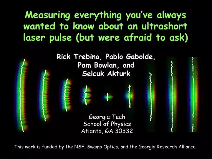
1. Measuring everything you’ve always wanted to know about an ultrashort laser pulse (but were afraid to ask) Rick Trebino, Pablo Gabolde, Pam Bowlan, and Selcuk Akturk Georgia Tech School of Physics Atlanta, GA 30332 This work is funded by the NSF, Swamp Optics, and the Georgia Research Alliance.

2. We desire the ultrashort laser pulse’s intensity and phase vs. time or frequency. Light has the time-domain spatio-temporal electric field: Intensity Phase (neglecting the negative-frequency component) Equivalently, vs. frequency: Spectral Spectrum Phase Knowledge of the intensity and phase or the spectrum and spectralphaseis sufficient to determine the pulse.

3. Frequency-Resolved Optical Gating (FROG) FROG is simply a spectrally resolved autocorrelation. This version uses SHG autocorrelation. Pulse to be measured Beam splitter Camera E(t–t) SHG crystal Spec- trometer E(t) Esig(t,t)= E(t)E(t-t) Variable delay, t FROG uniquely determines the pulse intensity and phase vs. time for nearly all pulses. Its algorithm is fast (20 pps) and reliable.

4. SHG FROG traces for various pulses Cubic-spectral-phase pulse Self-phase-modulated pulse Double pulse Intensity Frequency Time Frequency Frequency Delay Delay SHG FROG traces are symmetrical, so it has an ambiguity in the direction of time, but it’s easily removed.

5. SHG FROG trace with 1% additive noise FROG easily measures very complex pulses Occasionally, a few initial guesses are necessary, but we’ve never found a pulse FROG couldn’t retrieve. Red = correct pulse;Blue = retrieved pulse

6. FROG Measurements of a 4.5-fs Pulse! Baltuska, Pshenichnikov, and Weirsma, J. Quant. Electron., 35, 459 (1999). FROG is now even used to measure attosecond pulses.

7. GRating-Eliminated No-nonsense Observationof Ultrafast Incident Laser Light E-fields(GRENOUILLE) FROG 2 key innovations: Asingle optic that replaces the entiredelay line, and a thickSHG crystal that replaces both the thin crystal andspectrometer. GRENOUILLE P. O’Shea, M. Kimmel, X. Gu, and R. Trebino, Opt. Lett. 2001.

8. Pulse #1 Here, pulse #1 arrives earlier than pulse #2 x Here, the pulses arrive simultaneously Here, pulse #1 arrives later than pulse #2 Pulse #2 The Fresnel biprism Crossing beams at a large angle maps delay onto transverse position. Input pulse t = t(x) Fresnel biprism Even better, this design is amazingly compact and easy to use, and it never misaligns!

9. The thick crystal Very thin crystal creates broad SH spectrum in all directions. Standard autocorrelators and FROGs use such crystals. Thin crystal creates narrower SH spectrum in a given direction and so can’t be used for autocorrelators or FROGs. Thick crystal begins to separate colors. Thin SHG crystal Thick SHG crystal Very thick crystal acts like a spectrometer! Replace the crystal and spectrometer in FROG with a very thick crystal. Very thick crystal Suppose white light with a large divergence angle impinges on an SHG crystal. The SH wavelength generated depends on the angle. And the angular width of the SH beam created varies inversely with the crystal thickness. Very Thin SHG crystal

10. GRENOUILLE FROG Measured Retrieved Testing GRENOUILLE Compare a GRENOUILLE measurement of a pulse with a tried-and-true FROG measurement of the same pulse: Retrieved pulse in the time and frequency domains

11. GRENOUILLE FROG Measured Retrieved Testing GRENOUILLE Compare a GRENOUILLE measurement of a complex pulse with a FROG measurement of the same pulse: Retrieved pulse in the time and frequency domains

12. Spatio-temporal distortions Ordinarily, we assume that the electric-field separates into spatial and temporal factors (or their Fourier-domain equivalents): where the tilde and hat mean Fourier transforms with respect to t and x, y, z.

13. x z Angularlydispersed output pulse Prism Input pulse Angular dispersion is an example of a spatio-temporal distortion. In the presence of angular dispersion, the mean off-axis k-vector component kx0depends on frequency, w.

14. Tilted window Prism pair Input pulse Input pulse Spatially chirped output pulse Spatially chirped output pulse Another spatio-temporal distortion is spatial chirp (spatial dispersion). Prism pairs and simple tilted windows cause spatial chirp. The mean beam position, x0, depends on frequency, w.

15. Angularly dispersed pulse with spatial chirp and pulse-front tilt Angularly dispersed pulse with spatial chirp and pulse-front tilt Input pulse Input pulse Prism Grating And yet another spatio-temporal distortion is pulse-front tilt. Gratings and prisms cause both spatial chirp and pulse-front tilt. The mean pulse time, t0, depends on position, x.

16. Angular dispersion always causes pulse-front tilt! Angular dispersion: whereg = dkx0/dw Inverse Fourier-transforming with respect tokx, ky,andkzyields: using the shift theorem Inverse Fourier-transforming with respect tow-w0yields: using the inverse shift theorem which is just pulse-front tilt!

17. The combination of spatial and temporal chirp also causes pulse-front tilt. Spatially chirped pulse with pulse-front tilt, but no angular dispersion Dispersive medium Spatially chirped input pulse vg(red) > vg(blue) The theorem we just proved assumed no spatial chirp, however. So it neglects another contribution to the pulse-front tilt. The total pulse-front tilt is the sum of that due to dispersion and that due to this effect. Xun Gu, Selcuk Akturk, and Erik Zeek

18. General theory of spatio-temporal distortions To understand the lowest-order spatio-temporal distortions, assume a complex Gaussian with a cross term, and Fourier-transform to the various domains, recalling that complex Gaussians transform to complex Gaussians: Grad students: Xun Gu and Selcuk Akturk Pulse-front tilt Spatial chirp dropping the x subscript on the k Angular dispersion Time vs. angle

19. x z The imaginary parts of the pulse distortions: spatio-temporalphase distortions The imaginary part of Qxt yields: wave-front rotation. Wave-propagation direction The electric field vs. x and z. Red = +Black = -

20. x z The imaginary parts of the pulse distortions: spatio-temporalphase distortions The imaginary part ofRxw is wave-front-tilt dispersion. w1 Plots of the electric field vs. x and z for different colors. w2 w3 There are eight lowest-order spatio-temporal distortions, but only two independent ones.

21. The prism pulse compressor is notorious for introducing spatio-temporal distortions. Wavelength tuning Wavelength tuning Prism Prism Prism Prism Fine GDD tuning Wavelength tuning Wavelength tuning Coarse GDD tuning (change distance between prisms) Even slight misalignment causes all eight spatio-temporal distortions!

22. The two-prism pulse compressor is better, but still a bigproblem. Coarse GDD tuning Wavelength tuning Roof mirror Periscope Prism Prism Fine GDD tuning Wavelength tuning

23. Signal pulse frequency        2w+dw Frequency 2wdw Tilt in the otherwise symmetrical SHG FROG trace indicates spatial chirp! Delay -t0 +t0 Fresnel biprism GRENOUILLE measures spatial chirp.  SHG crystal Spatially chirped pulse -t0  +t0 

24. GRENOUILLE accurately measures spatial chirp. Measurements confirm GRENOUILLE’s ability to measure spatial chirp. Positive spatial chirp Spatio-spectral plot slope (nm/mm) Negative spatial chirp

25. Zero relative delay is off to side of the crystal Zero relative delay is in the crystal center Frequency An off-center trace indicates the pulse front tilt! 0 Delay GRENOUILLE measures pulse-front tilt. Fresnel biprism Tilted pulse front SHG crystal Untilted pulse front

26. GRENOUILLE accurately measures pulse-front tilt. Varying the incidence angle of the 4th prism in a pulse-compressor allows us to generate variable pulse-front tilt. Negative PFT Zero PFT Positive PFT

27. Focusing an ultrashort pulse can cause complex spatio-temporal distortions. In the presence of just some chromatic aberration, simulations predict that a tightly focused ultrashort pulse looks like this: Intensity vs. x & z (at various times) Focus x z Propagation direction Ulrike Fuchs Increment between images: 20 fs (6 mm). Measuring only I(t) at a focus is meaningless. We need I(x,y,z,t)!

28. Also, researchers now often use shaped pulses as long as ~20 ps with complex intensities and phases. Time So we’ll need to be able measure, not only the intensity, but also the phase, that is, E(x,y,z,t), for even complex focused pulses. And we’ll also need great spectral resolution for such long pulses. And the device(s) should be simple and easy to use!

29. We desire the ultrashort laser pulse’s intensity and phase vs. space and time or frequency. Light has the time-domain spatio-temporal electric field: Intensity Phase (neglecting the negative-frequency component) Equivalently, vs. frequency: Spectral Spectrum Phase Knowledge of the intensity and phase or the spectrum and spectralphaseis sufficient to determine the pulse.

30. Strategy Measure a spatially uniform (unfocused) pulse in time first. GRENOUILLE Then use it to help measure the more difficult one with a separate measurement device. STRIPED FISH SEA TADPOLE

31. Spectral Interferometry Measure the spectrum of the sum of a known and unknown pulse. Retrieve the unknown pulse E(w) from the cross term. ~ 1/T T Eunk Eref Frequency Eref Eunk Spectrometer Camera Beam splitter With a known reference pulse, this technique is known as TADPOLE (Temporal Analysis by Dispersing a Pair Of Light E-fields).

32. w0 w0 Frequency Frequency Retrieving the pulse in TADPOLE The “DC” term contains only spectra The “AC” terms contain phase information Interference fringes in the spectrum FFT “Time” 0 Filter out these two peaks Filter & Shift Spectrum The spectral phase difference is the phase of the result. IFFT Keep this one. “Time” 0 This retrieval algorithm is quick, direct, and reliable. It uniquely yields the pulse. Fittinghoff, et al., Opt. Lett. 21, 884 (1996).

33. FROG’s sensitivity: TADPOLE ‘s sensitivity: 1 zeptojoule = 10-21 J SI is very sensitive! 1 microjoule = 10-6 J 1 nanojoule = 10-9 J 1 picojoule = 10-12 J 1 femtojoule = 10-15 J 1 attojoule = 10-18 J TADPOLE has measured a pulse train with only 42 zeptojoules (42 x 10-21 J) per pulse.

34. ~ 100tp ~ wp /100 < tp > 10wp wp = pulse bandwidth; tp = pulse length Spectral Interferometry does not have the problems that plague SPIDER. Recently* it was shown that a variation on SI, called SPIDER, cannot accurately measure the chirp (or the pulse length). SPIDER’s cross-term cosine: Linear chirp (djunk/dww) and wT are both linear in w and so look the same. Worse, wT dominates, so T must be calibrated—and maintained—to six digits! Desired quantity This is very different from standard SI’s cross-term cosine: The linear term of junk is just the delay, T, anyway! *J.R. Birge, R. Ell, and F.X. Kärtner, Opt. Lett., 2006. 31(13): p. 2063-5.

35. Examples of ideal SPIDER traces Even if the separation, T, were known precisely, SPIDER cannot measure pulses accurately. These two pulses are very different but have very similar SPIDER traces. Intensity (%)

36. More ideal SPIDER traces Unless the pulses are vastly different, their SPIDER traces are about the same. Practical issues, like noise, make the traces even more indisting-uishable. Intensity (%)

37. Spectral Interferometry: Experimental Issues The interferometer is difficult to work with. Mode-matching is important—or the fringes wash out. Phase stability is crucial—or the fringes wash out. Unknown Spectrometer Beams must be perfectly collinear—or the fringes wash out. To resolve the spectral fringes, SI requires at least five times the spectrometer resolution.

38. SEA TADPOLE Camera x Cylindrical lens Spatially Encoded Arrangement (SEA) SEA TADPOLE usesspatial, instead of spectral, fringes. l Reference pulse Fibers Grating Grad student: Pam Bowlan Unknown pulse Spherical lens SEA TADPOLE has all the advantages of TADPOLE—and none of the problems. And it has some unexpected nice surprises!

39. Why is SEA TADPOLE a better design? Fibers maintain alignment. Our retrieval algorithm is single shot, so phase stability isn’t essential. Single mode fibers assure mode-matching. Collinearity is not only unnecessary; it’s not allowed. And the crossing angle is irrelevant; it’s okay if it varies. And any and all distortions due to the fibers cancel out!

40. We retrieve the pulse using spatial fringes, not spectral fringes, with near-zero delay. The beams cross, so the relative delay, T, varies with position, x. 1D Fourier Transform from x to k The delay is ~ zero, so this uses the full available spectral resolution!

41. SEA TADPOLE theoretical traces (mm) (mm)

42. More SEA TADPOLE theoretical traces (mm) (mm)

43. -8 -6 6 8 SEA TADPOLE measurements SEA TADPOLE has enough spectral resolution to measure a 14-ps double pulse.

44. An even more complex pulse… An etalon inside a Michelson interferometer yields a double train of pulses, and SEA TADPOLE can measure it, too.

45. SEA TADPOLE achieves spectral super-resolution! Blocking the reference beam yields an independent measurement of the spectrum using the same spectrometer. The SEA TADPOLE cross term is essentially the unknown-pulse complex electric field. This goes negative and so may not broaden under convolution with the spectrometer point-spread function.

46. SEA TADPOLE spectral super-resolution When the unknown pulse is much more complicated than the reference pulse, the interference term becomes: Sine waves are eigenfunctions of the convolution operator.

47. Scanning SEA TADPOLE: E(x,y,z,t) By scanning the input end of the unknown-pulse fiber, we can measure E(w) at different positions yielding E(x,y,z,ω). So we can measure focusing pulses!

48. E(x,y,z,t) for a theoretically perfectly focused pulse. E(x,z,t) Simulation Pulse Fronts Color is the instantaneous frequency vs. x and t. Uniform color indicates a lack of phase distortions.

49. Measuring E(x,y,z,t) for a focused pulse. Aspheric PMMA lens with chromatic (but no spherical) aberration and GDD. f = 50 mmNA = 0.03 Measurement 810 nm Simulation 790 nm

50. Spherical and chromatic aberration Singlet BK-7 plano-convex lens with spherical and chromatic aberration and GDD. f = 50 mmNA = 0.03 Measurement Simulation 810 nm 790 nm