Download
1 / 60
600 likes | 723 Views
Business Cycle Model. KW 28, 29. AS-AD Framework. Microeconomists use supply/demand framework for thinking about markets. Macroeconomists use Aggregate Supply/ Aggregate Demand as the central framework for thinking about business cycles.

E N D
Business Cycle Model KW 28, 29
AS-AD Framework • Microeconomists use supply/demand framework for thinking about markets. • Macroeconomists use Aggregate Supply/ Aggregate Demand as the central framework for thinking about business cycles. • AS/AD framework examines the relationship between the level of output (real GDP) and the aggregate price level (GDP deflator). • We use the AS/AD to show how different events will affect output & prices in the short run.
Long Run Aggregate Supply • Central pillar of AS-AD framework is the assumption that there is no long run relationship between prices and firms willingness to produce goods. • In the long run, a rise in average prices will affect the price level of outputs and inputs. For any individual firm, a price rise is no incentive to produce more if input prices rise also. • Long-run level of output determined by productivity and labor force participation is called trend output or potential output.
Aggregate Demand Curve P LRAS Y YP
Short Run Aggregate Supply In the short-run, there is thought to be a positive relationship between the aggregate price level and firms’ willingness to supply goods. Why is the Aggregate Supply Curve Upward Sloping? • For some firms, some input prices, particularly wages, will not rise with the general price level. • If wages are sticky, a rise in the price of goods reduces the real cost of hiring workers. Firms profit-maximizing output levels hire more workers, work their existing employees longer hours and produce more output.
Aggregate Demand Curve P LRAS SRAS Y YP
What causes SRAS to shift? • To maximize profits, firms will produce up to the scale that the price level compensates them for their costs. • If costs of production drop, output will increase at any price level • If costs of production rise, output will decrease at any price level.
Cost Shifters • Commodity & Oil Prices Energy is a commodity used by all production processes and is a cost factor. • Wage Levels Labor is by far the biggest cost for most sectors. • Productivity New inventions or techniques may reduce the need for labor and thereby reduce costs.
Short Run Aggregate Supply Curve • Oil Prices Fall • Wages Decline • Productivity Increases SRAS P SRAS′ Y
Potential Output • Potential output is not the maximum output possible for a country. • Potential output is the level of production when supply and demand are in equilibrium in labor market. • When output is higher than potential, it is because real labor costs/real wages are low so there is excess demand for labor. • Market forces will push wages up! • When output is lower than potential, real wages are high so labor is in excess supply. • Market forces will push wages down!
Aggregate Supply in Labor Market P • Excess • Supply in • Labor Market • Wages Fall • SRAS Shifts Out • Excess Demand • In • Labor Market • Wages Rise • SRAS Shifts In Y YP
Aggregate Demand Curve P LRAS SRAS Y YP
Aggregate Demand • There is a negative relationship between the price of a single good and demand ceteris parabis. If the price of a good is high relative to other goods, consumers will find substitutes. • Aggregate demand curve is the effect of the average price (in terms of money) on demand for all goods.
Aggregate Demand Curve P AD Y YLR
Why is the AD curve downward sloping? • Wealth Effect: increase in prices directly reduces purchasing power of consumers with savings in money assets. • Interest Rate Effect If prices go up, households & firms need more liquidity for spending on a given amount of goods. As consumers shift funds to cash, interest rate in capital markets will rise having negative impacts on demand for investment goods.
Cont. In HK, monetary policy is to have a fixed exchange rate with the US dollar. Interest rates are typically at US dollar levels. Take exchange rates as given: • International Trade Effect An increase in prices at a fixed exchange rate increases the relative costs of a countries exports and encourages domestic consumers to switch to imports.
Demand Matters • In the short-run, the position of the demand curve matters for equilibrium output. • Over time, the economy’s correction mechanism will restore the economy to a long-run in which the long-term supply factors determine output.
Short Run Equilibrium: Output Above Potential P SRAS Labor market displays excess demand P* A AD Y Y* YP
Long Run Equilibrium: SRAS shifts in as wages rise P SRAS P* B Wages rise and the profit maximizing production level falls. A AD Y YP
Short Run Equilibrium: Output Below Potential P SRAS Labor market displays excess supply P* A AD Y Y* YP
Long Run Equilibrium: SRAS shifts in as wages rise P Wages fall and the profit maximizing production level rises. SRAS SRAS ′ A P* B AD Y YP
Business Cycles • Economy has a self correcting mechanism, the labor market, that automatically returns the economy to the level of potential output in the long-run. • Demand is subject to fluctuations caused by external events. • Business cycles are the time between when a shock hits and when the self-correcting mechanism returns the economy to the long run. • The labor market is imperfect. Contracts and wages are renegotiated infrequently and matching between employers and employees is time-consuming.
Keynesian View of Business Cycles • Mainstream economic view is that shocks that affect the demand curve are the main driver of business cycles. • Demand is a positive feedback system and thus can be volatile. • In business cycles driven by demand shocks, prices rise during expansions and fall during recessions.
Demand Driven Boom SRAS′ P • Economy in LT equilibrium • Demand shifts out • Rising wages leads to return to equilibrium SRAS 3 P* 2 1 AD AD Y Y* YP
Demand Driven Recession P • Economy in LT equilibrium • Demand shifts in • Falling wages leads to return to equilibrium SRAS 1 2 P* 3 AD AD′ SRAS′ Y Y* YP
What causes the demand curve to shift? • Shifts in Household Consumption • 1) Wealth effect; 2) optimism about future; • Shifts in Corporate Investment Spending • 1) Interest Rates; 2) optimism about future • Shifts in Trade Balance • 1) Exchange Rates; 2) Foreign business cycles.
Income and Expenditure KW Chapter 28
Income and Expenditure • Two components of expenditure may depend strongly on income levels • Consumption • Imports • Net Exports = Exports – Imports: the trade balance is negatively impacted by domestic income. • To simplify, assume a zero trade balance and no government spending, NX = 0, G = 0
Consumption Function • Consumption is in the form • Where • A = Autonomous Consumption not directly dependent on current income • mpc = marginal propensity to consume the fraction of extra income that will go to spending • YD = Disposable Income
What causes the Consumption Function to shift? The determinants of autonomous income: • Real wealth – Stock or property market prices changes will shift A. • Expectations of Future Income – Optimism and pessimism of the household sector affects spending patterns.
Consumption Function Real Consumption ΔC ΔYD A Disposable Income
Shift Up in Consumption Function Real Consumption A' A Disposable Income
In Recent Years, the consumption function in HK has shifted down! 1998
Investment • We can divide investment into two categories: • Planned Fixed Investment: Building P&E for future production • Unplanned Inventory Investment
What causes Planned Investment to shift? • Changes in the Foreign Interest Rate– Real interest rate affects corporate investment spending, residential investment spending, consumer durables etc. • Expected Returns to Capital– Optimism and pessimism of the business sector affects spending patterns. • Capital Overhang – If firms have built up too much plant & equipment in a previous investment bubble, investment spending will decline.
Expenditure Curve Planned Expenditure C+IPlanned mpc A+IPlanned Income
Q: Why is demand so volatile?A: Demand is multiple feedback loop • Total Expenditure is an increasing function of aggregate income. Expenditure = C+I • Consumers will spend more if they have greater income. • But Expenditure creates production • Production creates income….
Expenditure =Income = GDP Planned Expenditure = Actual Expenditure Planned Expenditure IUnplanned C+IPlanned -IUnplanned 45º Income = Y = Expenditure
Expenditure =Income = GDP Planned Expenditure • Output above expenditure • Inventories increasing • Firms cut back on production • Reducing income levels. • Output below expenditure • Inventories declining • Firms increase production • Increasing income. C+I+G+NX 45º Y* Income
Autonomous Expenditure Increases Expenditure C+I A,I↑ Extra Expenditure Increases Output which increases income which increases expenditure which increases output which increases income … Multiplier effect Output 45º GDP Income
Multiplier Effect Firms mpc Savings Workers Spenders
Multiplier Effect Central Bank Firms mpc Workers Savings Spenders
Multiplier Effect Firms Savings mpc Workers Spenders
Multiplier • Expenditure = IPlanned+ A + mpc∙Income • GDP = IPlanned+ A + mpc∙GDP • (1-mpc)∙GDP = IPlanned+ A • GDP = [1/(1-mpc)] ∙ IPlanned+ A • Expenditure Multiplier = [1/(1-mpc)]
Open Economy Multiplier • The greater is the fraction of spending that is done on imports, the less income is recycled into extra spending on consumer goods. • mpc should be lower for very open economies (like HK) • Multiplier should be lower for very open economy.
Multiplier Effect Government Firms mpc Savings Workers Spenders Imports