Download
1 / 34
340 likes | 409 Views
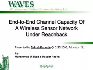
End-to-End Channel Capacity Of A Wireless Sensor Network Under Reachback. Presented by Shirish Karande @ CISS 2006, Princeton, NJ For Muhammad U. Ilyas & Hayder Radha. Objectives.

E N D
End-to-End Channel Capacity Of A Wireless Sensor Network Under Reachback Presented by Shirish Karande @ CISS 2006, Princeton, NJ For Muhammad U. Ilyas & Hayder Radha
Objectives • To determine an expression for the end-to-end channel capacity between a sensor and the base station of a 2-level hierarchy, Wireless Sensor Network employing Slepian-Wolf coding. • To determine the effects of cluster sizes on end-to-end capacity.
Outline • Network Model • Wireless Networking Standards for WSNs • End-to-End Channel • Notation • Cluster Communication Capacity • Overlay Network Communication Capacity • End-to-End Capacity • Results
Tesselated Wireless Sensor Networks • Gupta & Kumar † studied the scalability of a wireless networks with randomly chosen source destination pairs. • They offer two solutions; • Design smaller networks • Localize communication by clustering nodes. • Assumptions • Network has a 2-level hierarchy. • (Intra-)cluster communication between nodes and clusterhead (CLH) is 1-hop and proceeds at one frequency. • Different clusters may or may not use different frequencies. • ON communication proceeds at one frequency. __________________________________________________________________ † P. Gupta, and P. R. Kumar, “The Capacity of Wireless Networks,” IEEE Transactions on Information Theory, Vol. 46, No. 2, March 2000.
Cluster Communication Slepian-Wolf Coding for WSNs† • Basic Idea: • Sensors transmit readings to CLH one after the other. • Successive transmissions in a round will take fewer bits (figure). • Total number of bits transmitted will approach joint entropy. • Assumption: • Loss of the k-th transmission causes inability of receiver to reconstruct all following transmissions k+1 to n. • MAC protocol may be CSMA-CA or TDMA ___________________________________________________ † D. Marco, and D. L. Neuhoff, “Reliability vs. Efficiency in Distributed Source Coding for Field-Gathering Sensor Networks,” IEEE International Conference on Information Processing in Sensor Networks (IPSN’04), Berkeley, CA, 2004.
Overlay Network Communication • In the Overlay Network (ON), communication between CLHs and the BS proceeds over multihop routes (figure). • We are assuming use of a shortest path routing protocol that subsequently results a tree topology for the routes to BS (figure). • Transmissions in the ON are on one frequency, i.e. • Higher traffic volume near the base station gives rise to the reachback problem. • MAC protocol may be CSMA-CA or TDMA __________________________________________________________________ †J. Barros, S. D. Servetto, “On the Capacity of the Reachback Channel in Wireless Sensor Networks,” IEEE Workshop on Multimedia Signal Processing, December 2002.
End-to-End Channel Model Bit Error Rate & Packet Error Rate (end-to-end) Bit Error Rate & Packet Error Rate (1 hop) Bit Error Rate Pathloss Model
Notation Is the total number of sensors. Is the total number of clusters. Is the number of sensors in cluster i. Is the i-th cluster’s j-th node. Is the clusterhead (CLH) of cluster i. Is the frequency used for cluster communication in the i-th cluster.
Notation Is a function returning the spatial distance between i-th cluster’s j-th node and k-th cluster’s l-th node. Is the probability of nk(l) transmitting at the same time as ni(j) Is a function that returns the frequency at which the node provided as argument is communicating. • Is the indicator function returning; • 1 when the two nodes in the argument are communicating at the same frequency and there is a potential for interference. • 0 when the two nodes in the argument are communicating at different frequencies and there is NO potential for interference.
Pathloss Model • We are considering the pathloss (PL) model in the “IEEE 802.15.4a Channel Model - final report”† published by the IEEE 802.15.4a channel modeling subgroup that was subsequently adopted for all further work on this standard. • Separate channel models for • 100-900 MHz (indoor office) • 1000 MHz (narrowband) • 2 – 6 GHz (short range Body Area Networks) • 2 – 10 GHz (indoor residential, indoor office, industrial, outdoor, open outdoor) • All 3 wireless networking standards being considered fall in the 2.4 – 2.4835 GHz freq range. • Most envisioned WSN applications are expected to operate in environments considered for 2 – 10 GHz PL model. _________________________________________________________ †Andreas F. Molisch, Kannan Balakrishnan, Chia-Chin Chong, Shahriar Emami, Andrew Fort, Johan Karedal, Juergen Kunisch, Hans Schantz, Ulrich Schuster, Kai Siwiak, “IEEE 802.15.4a channel model - final report”, 2004.
2 – 10 GHz Pathloss Model • Provides the received signal power at the i-th cluster’s j-th node of a transmission from the k-th cluster’s l-th node is the transmitter signal power after amplification is the transmitter antenna efficiency is the receiver antenna efficiency These are assumed constant for all nodes in a WSN of homogeneous devices.
Pathloss Model • The pathloss model is accompanied with sets of values for its environmental parameters for the different environments mentioned previously. • However, some reference parameters remain constant across all environments, these are; Reference frequency Reference distance • Based on these parameters we can determine the different remaining model paramters;
Physical Layer Model • For the Physical Layer Channel Model we assume an Additive White Gaussian Noise (AWGN) channel that is characterized by the Signal-to-Interference & Noise-Ratio (SINR) at the receiver. is the ambient noise power due to co-located communication networks operating in same frequency spectrum, or devices (e.g. microwave ovens). Is the signal power of the transmitted signal at the receiver Is the signal power of interfering nodes at the receiver
Physical Layer Model • To obtain the SINR of the signal transmitted by the i-th cluster’s j-th node at its CLH (i.e. CLH of cluster i), we substitute the pathloss model in the power terms of the SINR equation.
Bit Error Rate Next, from our knowledge of a Physical Layer model we compute a Bit Error Rate (BER). We use the Lognormal Shadow Fading Model†. If, Then, ‡ ______________________________________________ † T.S. Rappaport, “Wireless Communications – Principles and Practice, 2nd ed,” Pearson Education, Singapore, 2002. ‡
Packet Error Rate • Recall:Failure of ni(0) to receive k-th transmission from a sensor in a round results in an inability to reconstruct/ a complete loss of all subsequent transmissions k+1 to Ni. Hence, † Is the number of header bits. _______________________________________________ †
Options in Overlay Network • We are considering two options for the way CLHs communicate their packets to the Base Station. • Option 1: No recoding, simple forwarding of downstream packets and transmission of own packets. • Option 2: Additional compression of own packet based on received downstream packets. ________________________________________ Downstream: farther away from base station Upstream: closer to base station
Pathloss Model (ON) • Remains similar to the one derived for the cluster-level communication, Is a function that returns the upstream neighbor of ni(0). Is a function that returns the set of all downstream neighbors of ni(0). If,
1-Hop Bit Error Rate (ON) • Similar to cluster-level BER model, the BER of the channel between ni(0) and its upstream neighbor is, • The expressions obtained up to this point hold true for ONs irrespective of whether or not CLHs are doing Slepian-Wolf recoding on their own packets based on packets received from downstream CLHs.
CLH-to-Base Station Bit Error Rate • The BER of the channel formed between a CLH and the base station can be treated as a cascade of BSCs. • The BER is defined by a recursive expression which models the channel as two BSCs (i) a BSC between the CLH and its upstream neighbor, and (ii) another BSC between the upstream neighbor and the Base station.
1-Hop Packet Error Rate Is the packet error rate for the link between nk(0) and R1↑(nk(0) for a packet originated at ni(0). For an ON without Slepian-Wolf coding. For an ON with Slepian-Wolf coding.
CLH-to-Base Station Packet Error Rate Is the end-to-end packet error model for the channel between CLH ni(0) and the base station. Is a function that returns the set of all downstream neighbors of ni(0). † ___________________________________________________________________________ †
Sensor-to-Base Station/ End-to-End BER & PER Is the packet error rate for the channel from ni(j) to ni(0) to base station. † Is the packet error rate for the channel from ni(j) to ni(0) to base station. ‡ _________________________________________________________________________ † ‡
Results • Physical layout and routing topology of a wireless sensor network consisting of 50 sensors in a square shaped plane of size 10 x 10. • Configured with 5 CLHs. • Base station is located at coordintate (0,0). • We assume an IEEE 802.15.4 frame structure.
End-to-End Channel Capacity and Probability Figure 1 - Bit and packet error probability of the end-to-end channel. Figure 2 – Bit and packet level capacity of the end-to-end channel.
Effect of Clustering on Capacity Figure 1 - Bit and packet error probability of the end-to-end channel with varying number of clusterheads. Figure 2 - Bit and packet level capacity of the end-to-end channel with varying number of clusterheads.
Thank You! ???
References • P. Gupta, and P. R. Kumar, “The Capacity of Wireless Networks,” IEEE Transactions on Information Theory, Vol. 46, No. 2, March 2000. • J. Barros, S. D. Servetto, “On the Capacity of the Reachback Channel in Wireless Sensor Networks,” IEEE Workshop on Multimedia Signal Processing, December 2002. • “IEEE P802.15.4/D18, Draft Standard: Low Rate Wireless Personal Area Networks,” February 2003. • Soo Young Shin, Hong Seong Park, Sunhyun Choi, Wook Hyun Kwon, "Packet Error Rate Analysis of IEEE 802.15.4 under IEEE 802.11b Interference," 3rd International Conference on Wired/ Wireless Internet Communications 2005 (WWIC'05), Xanthi, Greece, May 11-13, 2005. • Andreas F. Molisch, Kannan Balakrishnan, Chia-Chin Chong, Shahriar Emami, Andrew Fort, Johan Karedal, Juergen Kunisch, Hans Schantz, Ulrich Schuster, Kai Siwiak, “IEEE 802.15.4a channel model - final report,” 2004. • D. Marco, and D. L. Neuhoff, “Reliability vs. Efficiency in Distributed Source Coding for Field-Gathering Sensor Networks,” IEEE International Conference on Information Processing in Sensor Networks (IPSN’04), Berkeley, CA, 2004. • T.S. Rappaport, “Wireless Communications – Principles and Practice, 2nd ed,” Pearson Education, Singapore, 2002.