Download
1 / 1
10 likes | 100 Views
Initial testing of longwave parameterizations for broken water cloud fields - accounting for transmission Ezra E. Takara and Robert G. Ellingson Department of Meteorology, Florida State University, Tallahassee, FL 32306. Known overcast skies. Derived overcast. Results for May 30, 1999.

E N D
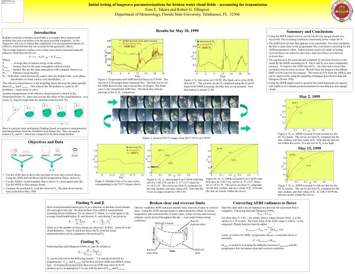
Initial testing of longwave parameterizations for broken water cloud fields - accounting for transmission Ezra E. Takaraand Robert G. Ellingson Department of Meteorology, Florida State University, Tallahassee, FL 32306 Known overcast skies Derived overcast Results for May 30, 1999 • Summary and Conclusions • Using the MWR liquid water to screen out the less opaque clouds was successful. The screening resulted in consistently lower values for N. • The AERI derived clear flux appears to be reasonable. For clear conditions the flux is quite close to the pyrgeometer flux even before correcting for the AERI-pyrgeometer offset. Improvements need to be made in finding overcast fluxes on relatively clear days, and clear fluxes on relatively overcast days. • The gap between the retrieved and computed Ne has been closed to some extent by the MWR screening for N. The N and Ne now have comparable accuracy. To improve the AERI derived Ne , the clear and overcast flux envelopes must be more accurate. Results from the longwave broadband QME will be used for this purpose. The retrieval of N from the ARSCL data can be improved by using the sampling techniques described in Han and Ellingson (Poster 18D). • Using the MWR liquid water to quantify the cloud transmissivity/opacity will enable us to evaluate parameterizations for non-black or non-opaque clouds. Introduction pyrgeometer TLVC Radiative transfer in broken cloud fields is a complex three dimensional problem that can overwhelm even the most powerful computers. In the longwave, one way to reduce this complexity is to use parameterizations of effective cloud fraction that can account for the geometric effects. The average longwave surface over a large area can be expressed using the effective cloud fraction (Ne) as: F = (1 – Ne) Fclear + Ne Fovercast Where, F - Average flux of radiant energy at the surface. Fclear - Surface flux for the same atmosphere without clouds. Fovercast - Surface flux for the same atmosphere with complete cloud cover. Ne - Effective cloud fraction Ne = f(absolute cloud fraction (N), aspect ratio (b), droplet radii, water phase, distribution of cloud, centers, size distribution, ...) The effective cloud fraction is the weighting factor between the plane parallel fluxes Fclear and Fovercast . This reduces the 3D problem to a pair of 1D problems -- much easier to solve. Another interpretation of the effective cloud fraction is shown in the illustration below; Ne takes into account the effect of the cloud thickness. As a result, Ne must be larger than the absolute cloud fraction (N). AERI radiance q q q q q Derived clear Known clear skies Time N < Ne Figure 1. Pyrgeometer and AERI derived fluxes on 5/30/99. The red curve is the pyrgeometer measured flux. The blue curves are the AERI derived clear and overcast flux envelopes. The black curve is the interpolated AERI flux. The black dots indicate intervals of the N, Ne comparison. Figure 2. Ne time series on 5/30/99. The black curve is the AERI derived Ne . The red dots are the Ne computed using the N and b found with MWR screening; the blue dots are unscreened. Note that sunrise is around 11:00. May 2, 1999 Here we present some preliminary findings based on longwave measurements and data products from the Southern Great Plains site. They are used to retrieve Ne and N -- which are compared to Ne from cloud models. Figure 6. Ne vs. MWR screened N with red dots for the (N, Ne) points. The curves are from Ne computed for the min, median, and max values of b. Note that the dots are not within the curves. N is too low or Ne is too high. Figure 3. Series of TLCV images from 20:57-22:01 on 5/30/99. Objectives and Data May 15, 1999 AERI MWR Ne N, b Figure 5a. Ne vs. unscreened N on 5/30/99 with blue dots for 3:40-3:54, red for 11:37-12:37, black for 21:14-21:18. The curves are from Ne computed for the min, median, and max values of b. Note that the N are too large except for 3:40-3:54. Figure 5b. Ne vs. MWR screened N on 5/30/99 with blue dots for 3:40-3:54, red for 11:37-12:37, black for 21:14-21:18. The curves are from Ne computed for the min, median, and max values of b. Note that the dots are mostly within the curves. Figure 4. Detailed view of Ne time series, corresponding to the TLCV images above. • Use the AERI data to derive the envelope of clear and overcast fluxes. Using the AERI derived fluxes and the pyrgeometer fluxes, derive Ne. • Use the ARSCL cloud boundary data to derive N, cloud aspect ratio (b). Use the MWR to find opaque clouds. • Compare the predicted Ne with the retrieved Ne. The data shown herein were collected in May 1999. Figure 7. Ne vs. MWR screened N with red dots for the (N, Ne) points. The curves are from Ne computed for the min, median, and max values of b. As with 5/30/99 the dots are mostly within the curves. Finding Ne Following Han and Ellingson (1999), Ne may be written as: Finding N and Most cloud parameterizations give Ne as a function of absolute cloud amount (N) and aspect ratio (b). We derived them from ARSCL measurements assuming frozen turbulence. For an interval T=10min, at a wind speed u, the average cloud length/radius, R, and fraction N seen during T are given as: Converting AERI radiances to fluxes Once the clear and overcast radiances are derived, the equivalent flux is computed. Following Han and Ellingson (1999), Broken clear and overcast limits The low variability AERI radiances identify time intervals of clear or overcast skies. Using the AERI measurements to approximate the effects of surface temperature and vertical profile of water vapor, values of clear and overcast radiance can be derived throughout the day -- even under broken cloud conditions. Ne can be retrieved in the following manner: F is measured directly by pyrgeometers. Fclear and Fovercast can be derived from AERI and ARSCL cloud base. Averaging the pyrgeometer data over an AERI time interval (8-10 minutes) gives an appropriate F to use with the derived Fclear and Fovercast . For clear skies L=3.45 -- for cloudy skies L ranges linearly from p at the surface to 3.25 at 6km. The lower limit of the AERI range is 520cm-1 so the integrated Planck function must be added: ARSCL where m is the number of times clouds are observed. =R/H ; where H is the cloud thickness. Once N and are fixed, the Ne from the cloud parameterization can be compared to the retrieved Ne . Lastly, to correct for AERI - pyrgeometer biases, a correction factor is necessary. dFoffset is found by averaging the difference between Funcorrected and the pyrgeometer flux for known clear and overcast conditions.