Download
1 / 1
10 likes | 115 Views
Numerics. y = sensor value x = ambiance value = time constant. special solution for x = const. :. Fig.2: measured (T), filtered (Tf) and reconstructed (Tx) Profiles of the Vaisala Sensor.

E N D
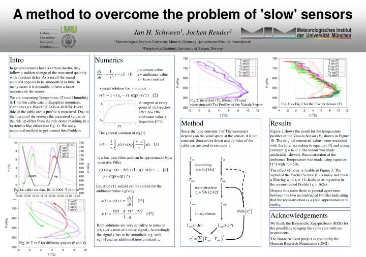
Numerics y = sensor value x = ambiance value = time constant special solution for x = const. : Fig.2: measured (T), filtered (Tf) and reconstructed (Tx) Profiles of the Vaisala Sensor A tangent at every point of y(t) reaches after t= the ambiance value x (equation [1*]). x Fig.3: as Fig.2 for the Fischer Sensor (F) y0 Method Since the time constant of Thermometers depends on the wind speed at the sensor, it is not constant. Successive down and up rides of the cable car are used to estimate : t/ The general solution of eq.[1] Tdn Tup is a low pass filter and can be aproximated by a recursive Filter smoothing f = 6s [14s] down up Tfdn Tfup Fig.1a: cable car data 10.12.2004 T vs time Equation [1] and [4] can be solved for the ambiance value x giving: reconstruction x = 50s [2:42] Txdn Txup Interpolation Txdn (i·P) Txup(i·P) Both solutions are very sensitive to noise in y(t) (derivation of a noisy signal). Accordingly the signal y has to be smoothed, e.g. with eq.[4] and an additional time constant f. Fig.1b: T vs P for different sensors (F and V) A method to overcome the problem of 'slow' sensorsJan H. Schween1, Jochen Reuder21Meteorological Institute University Munich, Germany , jan.schween@lrz.uni-muenchen.de 2Geophysical Institute, University of Bergen, Norway Intro In general sensors have a certain inertia, they follow a sudden change of the measured quantity with a certain delay. As a result the signal received appears to be smooothed in time. In many cases it is desirable to have a faster response of the sensor. We are measuring Temperature (T) and Humiditiy (rH) on the cable cars at Zugspitze mountain, Germany (see Poster EGU06-A-01076). Every ride of the cable cars a profile is measured. Due to the inertia of the sensors the measured values of the ride up differ from the ride down resulting in a hysteresis like effect (see fig. 1). We use a numerical method to get around this Problem. Results Figure 2 shows the result for the temperature profiles of the Vaisala Sensor (V) shown in Figure 1b. The original measured values were smoothed with the filter according to equation [4] and a time constant f = 6s (i.e. the sensor was made artificially slower). Reconstruction of the ambiance Temperature was made using equation [1*] with x = 50s. The effect of noise is visible in Figure 3: The signal of the Fischer Sensor (F) is noisy and even a filtering with f = 14s leads to strong noise in the reconstructed Profile (x = 162s). Despite this noise there is general agreement between the two reconstructed Profiles indicating that the reconstruction is a good approximation to reality. Acknowledgements We thank the Bayerische Zugspitzbahn (BZB) for the possibility to equip the cable cars with our instruments. The Bannerwolken project is granted by the German Research Foundation (DFG)