Download
1 / 34
340 likes | 365 Views
This comprehensive guide delves into elementary probability manipulations, multi-variant distributions, joint and marginal probabilities, conditional probabilities, and more. Learn about Bayesian rules, probabilistic inference methods, conditional independence, and efficient inference strategies.

E N D
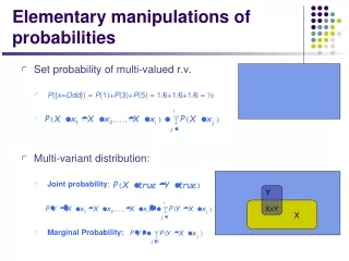
Elementary manipulations of probabilities • Set probability of multi-valued r.v. • P({x=Odd}) = P(1)+P(3)+P(5) = 1/6+1/6+1/6 = ½ • Multi-variant distribution: • Joint probability: • Marginal Probability: Y X∧Y X
Joint Probability • A joint probability distribution for a set of RVs gives the probability of every atomic event (sample point) • P(Flu,DrinkBeer) = a 2 × 2 matrix of values: • P(Flu,DrinkBeer, Headache) = ? • Every question about a domain can be answered by the joint distribution, as we will see later.
Conditional Probability • P(X|Y) = Fraction of worlds in which X is true that also have Y true • H = "having a headache" • F = "coming down with Flu" • P(H)=1/10 • P(F)=1/40 • P(H|F)=1/2 • P(H|F) = fraction of flu-inflicted worlds in which you have a headache = P(H∧F)/P(F) • Definition: • Corollary: The Chain Rule Y X∧Y X
MLE • Objective function: • We need to maximize this w.r.t. q • Take derivatives wrt q • Sufficient statistics • The counts, are sufficient statistics of data D or Frequency as sample mean
The Bayes Rule • What we have just did leads to the following general expression: This is Bayes Rule
More General Forms of Bayes Rule • P(Flu | Headhead ∧ DrankBeer) F B F B F∧H F∧H H H
Probabilistic Inference • H = "having a headache" • F = "coming down with Flu" • P(H)=1/10 • P(F)=1/40 • P(H|F)=1/2 • One day you wake up with a headache. You come with the following reasoning: "since 50% of flues are associated with headaches, so I must have a 50-50 chance of coming down with flu” Is this reasoning correct?
Probabilistic Inference • H = "having a headache" • F = "coming down with Flu" • P(H)=1/10 • P(F)=1/40 • P(H|F)=1/2 • The Problem: P(F|H) = ? F F∧H H
Prior Distribution • Support that our propositions about the possible has a "causal flow" • e.g., • Prior or unconditional probabilities of propositions e.g., P(Flu =true) = 0.025 and P(DrinkBeer =true) = 0.2 correspond to belief prior to arrival of any (new) evidence • A probability distribution gives values for all possible assignments: • P(DrinkBeer) =[0.01,0.09, 0.1, 0.8] • (normalized, i.e., sums to 1) F B H
Posterior conditional probability • Conditional or posterior (see later) probabilities • e.g., P(Flu|Headache) = 0.178 given that flu is all I know NOT “if flu then 17.8% chance of Headache” • Representation of conditional distributions: • P(Flu|Headache) = 2-element vector of 2-element vectors • If we know more, e.g., DrinkBeer is also given, then we have • P(Flu|Headache,DrinkBeer) = 0.070 This effect is known as explain away! • P(Flu|Headache,Flu) = 1 • Note: the less or more certain belief remains valid after more evidence arrives, but is not always useful • New evidence may be irrelevant, allowing simplification, e.g., • P(Flu|Headache,StealerWin) = P(Flu|Headache) • This kind of inference, sanctioned by domain knowledge, is crucial
Inference by enumeration • Start with a Joint Distribution • Building a Joint Distribution of M=3 variables • Make a truth table listing all combinations of values of your variables (if there are M Boolean variables then the table will have 2M rows). • For each combination of values, say how probable it is. • Normalized, i.e., sums to 1 B F H
B F H Inference with the Joint • One you have the JD you can ask for the probability of any atomic event consistent with you query
B F H Inference with the Joint • Compute Marginals
B F H Inference with the Joint • Compute Marginals
B F H Inference with the Joint • Compute Conditionals
B F H Inference with the Joint • Compute Conditionals • General idea: compute distribution on query variable by fixingevidence variables and summing over hidden variables
Summary: Inference by enumeration • Let X be all the variables. Typically, we want • the posterior joint distribution of the query variables Y • given specific values e for the evidence variables E • Let the hidden variables be H = X-Y-E • Then the required summation of joint entries is done by summing out the hidden variables: P(Y|E=e)=αP(Y,E=e)=α∑hP(Y,E=e, H=h) • The terms in the summation are joint entries because Y, E, and H together exhaust the set of random variables • Obvious problems: • Worst-case time complexity O(dn) where d is the largest arity • Space complexity O(dn) to store the joint distribution • How to find the numbers for O(dn) entries???
Conditional independence • Write out full joint distribution using chain rule: P(Headache;Flu;Virus;DrinkBeer) = P(Headache | Flu;Virus;DrinkBeer) P(Flu;Virus;DrinkBeer) = P(Headache | Flu;Virus;DrinkBeer) P(Flu | Virus;DrinkBeer) P(Virus | DrinkBeer)P(DrinkBeer) Assume independence and conditional independence = P(Headache|Flu;DrinkBeer) P(Flu|Virus) P(Virus)P(DrinkBeer) I.e., ? independent parameters • In most cases, the use of conditional independence reduces the size of the representation of the joint distribution from exponential in n to linear in n. • Conditional independence is our most basic and robust form of knowledge about uncertain environments.
Rules of Independence --- by examples • P(Virus | DrinkBeer) = P(Virus) iff Virus is independent ofDrinkBeer • P(Flu | Virus;DrinkBeer) = P(Flu|Virus) iff Flu is independent ofDrinkBeer, given Virus • P(Headache | Flu;Virus;DrinkBeer) = P(Headache|Flu;DrinkBeer) iff Headache is independent of Virus, given Flu and DrinkBeer
Marginal and Conditional Independence • Recall that for events E (i.e. X=x) and H (say, Y=y), the conditional probability of E given H, written as P(E|H), is P(E and H)/P(H) (= the probability of both E and H are true, given H is true) • E and H are (statistically) independent if P(E) = P(E|H) (i.e., prob. E is true doesn't depend on whether H is true); or equivalently P(E and H)=P(E)P(H). • E and F are conditionally independent given H if P(E|H,F) = P(E|H) or equivalently P(E,F|H) = P(E|H)P(F|H)
x Why knowledge of Independence is useful • Lower complexity (time, space, search …) • Motivates efficient inference for all kinds of queries Stay tuned !! • Structured knowledge about the domain • easy to learning (both from expert and from data) • easy to grow
Where do probability distributions come from? • Idea One: Human, Domain Experts • Idea Two: Simpler probability facts and some algebra e.g., P(F) P(B) P(H|¬F,B) P(H|F,¬B) … • Idea Three: Learn them from data! • A good chunk of this course is essentially about various ways of learning various forms of them!
Density Estimation • A Density Estimator learns a mapping from a set of attributes to a Probability • Often know as parameter estimation if the distribution form is specified • Binomial, Gaussian … • Three important issues: • Nature of the data (iid, correlated, …) • Objective function (MLE, MAP, …) • Algorithm (simple algebra, gradient methods, EM, …) • Evaluation scheme (likelihood on test data, predictability, consistency, …)
Parameter Learning from iid data • Goal: estimate distribution parameters q from a dataset of Nindependent, identically distributed (iid), fully observed, training cases D = {x1, . . . , xN} • Maximum likelihood estimation (MLE) • One of the most common estimators • With iid and full-observability assumption, write L(q) as the likelihood of the data: • pick the setting of parameters most likely to have generated the data we saw:
Example 1: Bernoulli model • Data: • We observed Niid coin tossing: D={1, 0, 1, …, 0} • Representation: Binary r.v: • Model: • How to write the likelihood of a single observation xi ? • The likelihood of datasetD={x1, …,xN}:
MLE for discrete (joint) distributions • More generally, it is easy to show that • This is an important (but sometimes not so effective) learning algorithm!
Example 2: univariate normal • Data: • We observed Niid real samples: D={-0.1, 10, 1, -5.2, …, 3} • Model: • Log likelihood: • MLE: take derivative and set to zero:
Overfitting • Recall that for Bernoulli Distribution, we have • What if we tossed too few times so that we saw zero head? We have and we will predict that the probability of seeing a head next is zero!!! • The rescue: • Where n' is know as the pseudo- (imaginary) count • But can we make this more formal?
The Bayesian Theory • The Bayesian Theory: (e.g., for dateD and modelM) P(M|D)= P(D|M)P(M)/P(D) • the posterior equals to the likelihood times the prior, up to a constant. • This allows us to capture uncertainty about the model in a principled way
Hierarchical Bayesian Models • q are the parameters for the likelihood p(x|q) • a are the parameters for the prior p(q|a) . • We can have hyper-hyper-parameters, etc. • We stop when the choice of hyper-parameters makes no difference to the marginal likelihood; typically make hyper-parameters constants. • Where do we get the prior? • Intelligent guesses • Empirical Bayes (Type-II maximum likelihood) computing point estimates of a :
Bayesian estimation for Bernoulli • Beta distribution: • Posterior distribution of q: • Notice the isomorphism of the posterior to the prior, • such a prior is called aconjugate prior
Bayesian estimation for Bernoulli, con'd • Posterior distribution of q: • Maximum a posteriori (MAP) estimation: • Posterior mean estimation: • Prior strength: A=a+b • A can be interoperated as the size of an imaginary data set from which we obtain the pseudo-counts Bata parameters can be understood as pseudo-counts
Effect of Prior Strength • Suppose we have a uniform prior (a=b=1/2), and we observe • Weak prior A = 2. Posterior prediction: • Strong prior A = 20. Posterior prediction: • However, if we have enough data, it washes away the prior. e.g., . Then the estimates under weak and strong prior are and , respectively, both of which are close to 0.2
Bayesian estimation for normal distribution • Normal Prior: • Joint probability: • Posterior: Sample mean