Download
1 / 27
270 likes | 436 Views
Analysis of variance (2). Lecture 10. Measurements (data). Descriptive statistics. Data transformation. Normality Check Frequency histogram (Skewness & Kurtosis) Probability plot, K-S test. YES. NO. Mean, SD, SEM, 95% confidence interval. Median, range, Q1 and Q3.

E N D
Analysis of variance (2) Lecture 10
Measurements (data) Descriptive statistics Data transformation Normality Check Frequency histogram (Skewness & Kurtosis) Probability plot, K-S test YES NO Mean, SD, SEM, 95% confidence interval Median, range, Q1 and Q3 Data transformation Fmax test Check the Homogeneity of Variance Non-Parametric Test(s) For 2 samples: Mann-Whitney For 2-paired samples: Wilcoxon For >2 samples: Kruskal-Wallis Sheirer-Ray-Hare NO K-W test, Dunn’s test One-way ANOVA Tukey’s test Two-way ANOVA YES Parametric Tests Student’s t tests for 2 samples; ANOVA for 2 samples; post hoc tests for multiple comparison of means
Kruskal-Wallis test with tied ranks • Example 10.11 (Zar, 1999) – comparison of pH among 4 ponds N = 8 + 8 + 7 + 8 = 31 H = {12/[N(N + 1)]} (Ri2/ni) - 3(N + 1) H = {12/[31(31 + 1)]} (8917.8) - 3(31 + 1) = 11.876 Number of groups of tied ranks = m = 7 T = (ti3 - ti) = (23 - 2) + (33 - 3) + (33 - 3) + (43 - 4) + (33 - 3) + (23 - 2) + (33 - 3) = 168 C = 1 - T / (N3 - N)= 1 - (168/ (313 - 31)) =0.9944 Hc = H/C = 11.876/ 0.9944 = 11.943 = k - 1 = 4 -1 = 3 20.05, 3 = 7.815 < 11.943, 0.005< p <0.01, hence reject Ho (Table B1)
Nonparametric multiple comparisons: Dunn’s test (e.g. 11.10, Zar 1999) Dunn’s test is a non-parametric test and is used to compare any significant different means or medians. Using Example 10.11: T = 168 For nA = 8 and nB = 8, SE = {[(N(N + 1)/12) – T /(12(N – 1)][(1/nA) + (1/nB)]} SE = {[(31(32)/12) – 168 /(12(31 – 1)][(1/8) + (1/8)]} = 4.53 For nA = 7 and nB = 8, SE = {[(31(32)/12) – 168 /(12(31 – 1)][(1/7) + (1/8)]} = 4.69 Sample ranked by mean rank: 1 2 4 3 Rank sum: 55 132.5 163.5 145 Sample sizes: 8 8 8 7 Mean ranks: 6.88 16.56 20.44 20.71 Similar to Tukey’s test In conclusion, water pH is the same in ponds 4 & 3 but is different in pond 1, and the relationship of pond 2 to the others is unclear. (see Table B15 for critical Q values)
Measurements (data) Descriptive statistics Data transformation Normality Check Frequency histogram (Skewness & Kurtosis) Probability plot, K-S test YES NO Mean, SD, SEM, 95% confidence interval Median, range, Q1 and Q3 Data transformation Fmax test Check the Homogeneity of Variance Non-Parametric Test(s) For 2 samples: Mann-Whitney For 2-paired samples: Wilcoxon For >2 samples: Kruskal-Wallis Sheirer-Ray-Hare NO K-W test, Dunn’s test Friedman One-way ANOVA Tukey’s test Two-way ANOVA YES Other ANOVAs Parametric Tests Student’s t tests for 2 samples; ANOVA for 2 samples; post hoc tests for multiple comparison of means Next lecture
Two-factor ANOVA • 2-way ANOVA • Can simultaneously assess the effects of two factors on a variable. • Can also test for interaction among factors, provided that data in each cell of a contingency table consist observations n > 1. • Assumption: normal data with equal variances but ANOVA is robust (see p. 185-188, Zar 1999)
2-way ANOVA with equal replication Example 12.1: The effects of sex and hormone treatment on plasma calcium concentrations (in mg/100 ml) of birds. • Questions: • Is there a significant difference between the mean calcium concentration of males and females? • Is there a significant difference between the mean calcium concentration in each treatment (control vs. hormone treatment)?
Passed the Fmax test, indicating equal variances among the four means • Mean and • 95% C.I. • Two factors • Sex • Hormone
SS total = SS within cells + SS between A + SS between B + SS interaction SS within cells = SS total – SS cells SS interaction = SS cells – SS between A – SS between B DF total = N – 1 DF cells (explained) = (nA)(nB) – 1 DF within cells (residual or error) = (nA)(nB)(n’ – 1) where n’= no. of replicates within each cell DF between A = nA – 1 DF between B = nB – 1 DF A B interaction = (DF between A)(DF between B)
SS total = 11354.3 – (436.5)2/20 = 1827.7 DF total = 20 – 1 = 19 • SS cells = [(74.4)2 + (60.6)2 + (162.6)2 + (138.9)2]/5 - (436.5)2/20 = 1461.3 DF cells = (2)(2) - 1 = 3 • SS within cells = SS total - SS cells = 1827.7 – 1461.3 = 366.4 DF within cells = (2)(2)(5 – 1) = 16
SS total = 11354.3 – (436.5)2/20 = 1827.7 DF total = 20 – 1 = 19 • SS cells = [(74.4)2 + (60.6)2 + (162.6)2 + (138.9)2]/5 - (436.5)2/20 = 1461.3 DF cells = (2)(2) - 1 = 3 • SS within cells = 1827.7 – 1461.3 = 366.4 DF within cells = (2)(2)(5 – 1) = 16 SS between treatments = {[(135.0)2 + (301.5)2] /(2)(5)} - (436.5)2/20 = 1386.1 DF between treatment = 2 - 1 = 1 SS between sexes = {[(237.0)2 + (199.5)2] /(2)(5)} - (436.5)2/20 = 70.31 DF between sexes = 2 - 1 = 1 SS interaction = SS cells – SS between A – SS between B = 1461.3 – 1386.1 – 70.31 = 4.900 DF interaction = (1)(1) = 1 Equations: See p. 242 (Zar, 1999)
Analysis of Variance Summary Table • There was a significant effect of hormone treatment on plasma calcium concentrations in the birds (P <0.001). • There was no interaction between sex and hormone treatment while the sex effect was not significant (likely due to inadequate power) Tukey test same as 1-way ANOVA
[Ca] [Ca] female male Sex Horm. Sex X Horm. control control hormone treated hormone treated [Ca] [Ca] Sex Horm. X Sex X Horm. X control control hormone treated hormone treated
[Ca] [Ca] Sex Horm. Sex Horm. Intera. female male control control hormone treated hormone treated [Ca] [Ca] Sex Horm. Intera. Sex Horm. Intera. control control hormone treated hormone treated
Interactive effects between variables: (a) no interaction; (b) interaction. (b) (a)
An example: The effects of light and sex on food intake in starlings. Total food intake (g) for 7 days
An example: The effects of light and sex on food intake in starlings. Two sexes have different food intake levels (p < 0.001). A significant interaction (p <0.05) indicates that two sexes respond significantly differently to day-length in the amount of food they eat.
Computation of the F statistics for tests of significance in 2-way ANOVA with replicates
2-way ANOVA for data without replication Interactioncannot be measured where data in each cell of a contingency table consist of single observations. Variability due to interaction is combined with the within variability and it is assumed to be negligible.
The randomized block See Example 12.4 (Zar, 99) Each block contains 4 animals: Repeated-measures See Example 12.5 (Zar, 1999) e.g. effects of diet type on food wastage in fish farm Other two experimental design suitable for 2-way ANOVA Other example: different colours of buckets (water traps) to sample insects Equivalent non-parametric method: Friedman’s analysis of variance by ranks (see p. 263-266, Zar 1999)
Use SPSS to conduct a 2-way ANOVA Dependent variable Factor A Factor B Column 1 Column 2 Column 3 obs. 1 1 1 obs. 2 1 2 obs. 3 1 3 obs. i - 2 2 1 obs. i - 1 2 2 obs. i 2 3 …….. …….. ……..
Measurements (data) Descriptive statistics Data transformation Normality Check Frequency histogram (Skewness & Kurtosis) Probability plot, K-S test YES NO Mean, SD, SEM, 95% confidence interval Median, range, Q1 and Q3 Data transformation Fmax test Check the Homogeneity of Variance Non-Parametric Test(s) For 2 samples: Mann-Whitney For 2-paired samples: Wilcoxon For >2 samples: Kruskal-Wallis Sheirer-Ray-Hare NO K-W test, Dunn’s test Friedman One-way ANOVA Tukey’s test Two-way ANOVA YES Other ANOVAs Parametric Tests Student’s t tests for 2 samples; ANOVA for 2 samples; post hoc tests for multiple comparison of means Next lecture
Key notes • After performing a Kruskal-Wallis test, a Dunn’s test can be used to identify any significantly different medians (or means) based on ranking • Two-way ANOVA can be used to analyze samples which have been subjected to two levels of treatment • In two-way ANOVA, there are several different design: (Model 1) both factors A and B are fixed factors; (Model 2) both factors are random factors; (Model 3) mixed factors. Furthermore, two-way ANOVA can also be applied to data with randomized block or repeated measure designs as well as data without replication. • In two-way ANOVA, interaction cannot be tested where data in each cell of a contingency table consist of single observations.