Download
1 / 10
140 likes | 622 Views
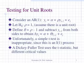
Testing for Unit Roots. Consider an AR(1): y t = a + r y t-1 + e t Let H 0 : r = 1, (assume there is a unit root) Define q = r – 1 and subtract y t-1 from both sides to obtain D y t = a + q y t-1 + e t

E N D
Testing for Unit Roots • Consider an AR(1): yt = a + ryt-1 + et • Let H0: r = 1, (assume there is a unit root) • Define q = r – 1 and subtract yt-1 from both sides to obtain Dyt = a + qyt-1 + et • Unfortunately, a simple t-test is inappropriate, since this is an I(1) process • A Dickey-Fuller Test uses the t-statistic, but different critical values Economics 20 - Prof. Anderson
Testing for Unit Roots (cont) • We can add p lags of Dyt to allow for more dynamics in the process • Still want to calculate the t-statistic for q • Now it’s called an augmented Dickey-Fuller test, but still the same critical values • The lags are intended to clear up any serial correlation, if too few, test won’t be right Economics 20 - Prof. Anderson
Testing for Unit Roots w/ Trends • If a series is clearly trending, then we need to adjust for that or might mistake a trend stationary series for one with a unit root • Can just add a trend to the model • Still looking at the t-statistic for q, but the critical values for the Dickey-Fuller test change Economics 20 - Prof. Anderson
Spurious Regression • Consider running a simple regression of yt on xt where yt and xt are independent I(1) series • The usual OLS t-statistic will often be statistically significant, indicating a relationship where there is none • Called the spurious regression problem Economics 20 - Prof. Anderson
Cointegration • Say for two I(1) processes, yt and xt, there is a b such that yt – bxt is an I(0) process • If so, we say that y and x are cointegrated, and call b the cointegration parameter • If we know b, testing for cointegration is straightforward if we define st = yt – bxt • Do Dickey-Fuller test and if we reject a unit root, then they are cointegrated Economics 20 - Prof. Anderson
Cointegration (continued) • If b is unknown, then we first have to estimate b , which adds a complication • After estimating b we run a regression of Dût on ût-1 and compare t-statistic on ût-1 with the special critical values • If there are trends, need to add it to the initial regression that estimates b and use different critical values for t-statistic on ût-1 Economics 20 - Prof. Anderson
Forecasting • Once we’ve run a time-series regression we can use it for forecasting into the future • Can calculate a point forecast and forecast interval in the same way we got a prediction and prediction interval with a cross-section • Rather than use in-sample criteria like adjusted R2, often want to use out-of-sample criteria to judge how good the forecast is Economics 20 - Prof. Anderson
Out-of-Sample Criteria • Idea is to note use all of the data in estimating the equation, but to save some for evaluating how well the model forecasts • Let total number of observations be n + m and use n of them for estimating the model • Use the model to predict the next m observations, and calculate the difference between your prediction and the truth Economics 20 - Prof. Anderson
Out-of-Sample Criteria (cont) • Call this difference the forecast error, which is ên+h+1 for h = 0, 1, …, m • Calculate the root mean square error (RMSE) Economics 20 - Prof. Anderson
Out-of-Sample Criteria (cont) • Call this difference the forecast error, which is ên+h+1 for h = 0, 1, …, m • Calculate the root mean square error and see which model has the smallest, where Economics 20 - Prof. Anderson