Download
1 / 34
340 likes | 375 Views
Lesson 50 – Area Between Curves. HL Math- Santowski. FAST FIVE. True or false & explain your answer:. Fast Five. 1. Graph 2. Integrate 3. Integrate 4. Evaluate. Lesson Objectives. 1. Determine total areas under curves 2. Apply definite integrals to a real world problems.

E N D
Lesson 50 – Area Between Curves HL Math- Santowski HL Math - Santowski
FAST FIVE True or false & explain your answer: HL Math - Santowski
Fast Five • 1. Graph • 2. Integrate • 3. Integrate • 4. Evaluate HL Math - Santowski
Lesson Objectives • 1. Determine total areas under curves • 2. Apply definite integrals to a real world problems HL Math - Santowski
(A) APPLICATIONS OF DEFINITE INTEGRALS – MOTION PROBLEMS 1. An object starts at the origin and moves along the x-axis with a velocity v(t) = 10t - t2 for 0 <t< 10 (a) What is the position of the object at any time, t ? (b) What is the position of the object at the moment when it reaches its maximum velocity? (c) How far has the object traveled before it starts to decelerate? HL Math - Santowski
(A) APPLICATIONS OF DEFINITE INTEGRALS – MOTION PROBLEMS 1. For the velocity functions given below for a particle moving along a line, determine the distance traveled and displacement of the particle: (a) v(t) = 3t – 5, 0 <t< 3 (b) v(t) = t2 – 2t – 8, 1 <t< 6 2. The acceleration function and the initial velocity are given for a particle moving along a line. Determine (a) the velocity at time t and (b) the distance traveled during the given time interval: (a) a(t) = t + 4, v(0) = 5, 0 <t< 10 (b) a(t) = 2t + 3, v(0) = -4, 0 <t< 3 HL Math - Santowski
(A) APPLICATIONS OF DEFINITE INTEGRALS – MOTION PROBLEMS Two cars, who are beside each other, leave an intersection at the same instant. They travel along the same road. Car A travels with a velocity of v(t) = t2 – t – 6 m/s while Car B travels with a velocity of v(t) = 0.5t + 2 m/s. (a) What are the initial velocities of the cars? (b) How far has each car gone after 4 seconds have elapsed? (c) When are the two cars beside each other again (i.e. when does the trailing car catch up to the leading car?) HL Math - Santowski
(B) General formula • To find the area between 2 curves, we use the general formula • Given that are continuous on [a,b] and that HL Math - Santowski
(C) Examples Sketch the curve of f(x) = x3 – x4 between x = 0 and x = 1. (a) Draw a vertical line at x = k such that the region between the curve and axis is divided into 2 regions of equal area. Determine the value of k. (b) Draw a horizontal line at y = h such that the region between the curve and axis is divided into 2 regions of equal area. Estimate the value of h. Justify your estimation. HL Math - Santowski
(C) Examples • (a) Find the area bounded by • (b) Find the area between the curves • (c) Find the region enclosed by • (d) Find the region enclosed by HL Math - Santowski
(D) Area Under VT Graphs Let’s deal with a journey of two cars as illustrated by their VT graphs We will let the two cars start at the same spot Here is the graph for Car 1 Highlight, calculate & interpret: The equation is HL Math - Santowski
(D) Area Under VT Graphs • Let’s deal with a journey of two cars as illustrated by their VT graphs • We will let the two cars start at the same spot • Here is the graph for Car 1I • Calculate, highlight & interpret: • The equation is HL Math - Santowski
(D) Area Under VT Graphs • Now let’s add a new twist to this 2 car problem: • Highlight, calculate and interpret: • Here are the two graphs: HL Math - Santowski
(D) Area Under VT Graphs Final question about the 2 cars: When do they meet again (since we have set the condition that they started at the same point) Explain how and why you set up your solution Here are the graphs again: HL Math - Santowski
(E) Economics Applications Now let’s switch applications to economics Our two curves will represent a marginal cost function and a marginal revenue function The equations are: Here are the two curves HL Math - Santowski
(E) Economics Applications Highlight, calculate and evaluate the following integrals: Here are the 2 functions: HL Math - Santowski
(E) Economics Applications Highlight, calculate and evaluate the following integrals: Here are the 2 functions: HL Math - Santowski
(E) Economics Applications So the final question then is how much profit did the company make between months 1 and 10? The 2 functions HL Math - Santowski
Lesson 50b - AVERAGE VALUE OF A FUNCTION Calculus - Santowski HL Math - Santowski
Lesson Objectives HL Math - Santowski 1. Understand average value of a function from a graphic and algebraic viewpoint 2. Determine the average value of a function 3. Apply average values to a real world problems
Fast Five HL Math - Santowski 1. Find the average of 3,7,4,12,5,9 2. If you go 40 km in 0.8 hours, what is your average speed? 3. How far do you go in 3 minutes if your average speed was 600 mi/hr 4. How long does it take to go 10 kilometers at an average speed of 30 km/hr?
(A) Average Speed • Suppose that the speed of an object is given by the equation v(t) = 12t-t2 where v is in meters/sec and t is in seconds. How would we determine the average speed of the object between two times, say t = 2 s and t = 11 s HL Math - Santowski
(A) Average Velocity HL Math - Santowski So, let’s define average as how far you’ve gone divided by how long it took or more simply displacement/time which then means we need to find the displacement. HOW?? We can find total displacement as the area under the curve and above the x-axis => so we are looking at an integral of Upon evaluating this definite integral, we get
(A) Average Value • If the total displacement is 261 meters, then the average speed is 261 m/(11-2)s = 29 m/s • We can visualize our area of 261 m in a couple of ways: (i) area under v(t) or (ii) area under v = 29 m/s HL Math - Santowski
(A) Average Velocity HL Math - Santowski So our “area” or total displacement is seen from 2 graphs as (i) area under the original graph between the two bounds and then secondly as (ii) the area under the horizontal line of v = 29 m/s or rather under the horizontal line of the average value So in determining an average value, we are simply trying to find an area under a horizontal line that is equivalent to the area under the curve between two specified t values So the real question then comes down to “how do we find that horizontal line?”
(B) Average Temperature • So here is a graph showing the temperatures of Toronto on a minute by minute basis on April 3rd. • So how do we determine the average daily temperature for April 3rd? HL Math - Santowski
(B) Average Temperature HL Math - Santowski So to determine the average daily temperature, we could add all 1440 (24 x 60) times and divide by 1440 possible but tedious What happens if we extended the data for one full year (525960 minutes/data points) So we need an approximation method
(B) Average Temperature HL Math - Santowski So to approximate: (1) divide the interval (0,24) into n equal subintervals, each of width x = (b-a)/n (2) then in each subinterval, choose x values, x1, x2, x3, …, xn (3) then average the function values of these points: [f(x1) + f(x2) + ….. + f(xn)]/n (4) but n = (b-a)/ x (5) so f(x1) + f(x2) + ….. + f(xn)/((b-a)/x) (6) which is 1/(b-a) [f(x1)x + f(x2)x + ….. + f(xn)x] (7) so we get 1/(b-a)f(xi)x
(B) Average Temperature HL Math - Santowski Since we have a sum of Now we make our summation more accurate by increasing the number of subintervals between a & b: Which is of course our integral
(B) Average Temperature HL Math - Santowski So finally, average value is given by an integral of So in the context of our temperature model, the equation modeling the daily temperature for April 3 in Toronto was Then the average daily temp was
(C) Examples HL Math - Santowski Find the average value of the following functions on the given interval
(D) Mean Value Theorem of Integrals HL Math - Santowski Given the function f(x) = 1+x2 on the interval [-1,2] (a) Find the average value of f(x) Question is there a number in the interval at x = c at which the function value at c equals the average value of the function? So we set the equation then as f(c) = 2 and solve 2 = 1+c2 Thus, at c = +1, the function value is the same as the average value of the function
(D) Mean Value Theorem of Integrals • Our solution to the previous question is shown in the following diagram: HL Math - Santowski
(E) Examples • For the following functions, determine: • (a) the average value on the interval • (b) Determine c such that fc = fave • (c) Sketch a graph illustrating the two equal areas (area under curve and under rectangle) HL Math - Santowski