Download
1 / 14
140 likes | 311 Views
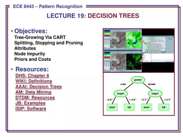
LECTURE 19: DECISION TREES. Objectives: Tree-Growing Via CART Splitting, Stopping and Pruning Attributes Node Impurity Priors and Costs Resources: DHS: Chapter 8 WIKI : Definitions AAAI: Decision Trees AM: Data Mining DTDM: Resources JB: Examples ISIP: Software. Overview.

E N D
LECTURE 19: DECISION TREES • Objectives:Tree-Growing Via CARTSplitting, Stopping and PruningAttributesNode ImpurityPriors and Costs • Resources:DHS: Chapter 8WIKI: DefinitionsAAAI: Decision TreesAM: Data MiningDTDM: ResourcesJB: ExamplesISIP: Software
Overview • Previous techniques have consisted of real-valued feature vectors (or discrete-valued) and natural measures of distance (e.g., Euclidean). • Consider a classification problem that involves nominal data – data described by a list of attributes (e.g., categorizing people as short or tall using gender, height, age, and ethnicity). • How can we use such nominal data for classification? How can we learn the categories of such data? Nonmetric methods such as decision trees provide a way to deal with such data. • Decision trees attempt to classify a patternthrough a sequence of questions. Forexample, attributes such as gender andheight can be used to classify people asshort or tall. But the best threshold forheight is gender dependent. • A decision tree consists of nodes and leaves, with each leaf denoting a class. • Classes (tall or short) are the outputs of the tree. • Attributes (gender and height) are a set of features that describe the data. • The input data consists of values of the different attributes. Using these attribute values, the decision tree generates a class as the output for each input data.
Basic Principles • The top, or first node, is called the root node. • The last level of nodes are the leaf nodesand contain the final classification. • The intermediate nodes are thedescendant or “hidden” layers. • Binary trees, like the one shown to theright, are the most popular type of tree.However, M-ary trees (M branches at each node) are possible. • Nodes can contain one more questions. In a binary tree, by convention if the answer to a question is “yes”, the left branch is selected. Note that the same question can appear in multiple places in the network. • Decision trees have several benefits over neural network-type approaches, including interpretability and data-driven learning. • Key questions include how to grow the tree, how to stop growing, and how to prune the tree to increase generalization. • Decision trees are very powerful and can give excellent performance on closed-set testing. Generalization is a challenge.
Nonlinear Decision Surfaces • Decision trees can produce nonlinear decision surfaces: • They are an attractive alternative to other classifiers we have studied because they are data-driven and can give arbitrarily high levels of precision on the training data. • But… generalization becomes a challenge.
Classification and Regression Trees (CART) • Consider a set D of labeled training data and a set of properties(or questions), T. • How do we organize the tree to produce the lowest classification error? • Any decision tree will successively split the data into smaller and smaller subsets. It would be ideal if all the samples associated with a leaf node were from the small class. Such a subset, or node, is considered pure in this case. • A generic tree-growing methodology, known as CART, successively splits nodes until they are pure. Six key questions: • Should the questions be binary (e.g., is gender male or female) or numeric (e.g., is height >= 5’4”) or multi-valued (e.g., race)? • Which properties should be tested at each node? • When should a node be declared a leaf? • If the tree becomes too large, how can it be pruned? • If the leaf node is impure, what category should be assigned to it? • How should missing data be handled?
Entropy-Based Splitting Criterion • We prefer trees that are simple and compact. Why? (Hint: Occam’s Razor). • Hence, we seek a property query, Ti, that splits the data at a node to increase the purity at that node. Let i(N) denote the impurity of a node N. • To split data at a node, we need to find the question that results in the greatest entropy reduction (removes uncertainty in the data): • Note this will peak when the two classes are equally likely (same size).
Alternate Splitting Criteria • Variance impurity: • because this is related to the variance of a distribution associated with the two classes. • Gini Impurity: • The expected error rate at node N if the category label is selected randomly from the class distribution present at node N. • Misclassification impurity: • measures the minimum probability that a training pattern would be misclassified at node N. • In practice, simple entropy splitting (choosing the question that splits the data into two classes of equal size) is very effective.
Choosing A Question • An obvious heuristic is to choose the query that maximizes the decrease in impurity: • where NL and NR are the left and right descendant nodes, i(NL) and i(NR) are their respective impurities, and PL is the fraction of patterns at node N that will be assigned to NL when query Ti is chosen. • This approach is considered part of a class of algorithms known as “greedy.” • Note this decision is “local” and does not guarantee an overall optimal tree. • A multiway split can be optimized using the gain ratio impurity: • where Pk is the fraction of training patterns sent to node Nk, and B is the number of splits, and:
When To Stop Splitting • If we continue to grow the tree until each leaf node has the lowest impurity, then the data will be overfit. • Two strategies: (1) stop tree from growing or (2) grow and then prune the tree. • A traditional approach to stopping splitting relies on cross-validation: • Validation: train a tree on 90% of the data and test on 10% of the data (referred to as the held-out set). • Cross-validation: repeat for several independently chosen partitions. • Stopping Criterion: Continue splitting until the error on the held-out data is minimized. • Reduction In Impurity: stop if the candidate split leads to a marginal reduction of the impurity (drawback: leads to an unbalanced tree). • Cost-Complexity: use a global criterion function that combines size and impurity: . This approach is related to minimum description length when the impurity is based on entropy. • Other approaches based on statistical significance and hypothesis testing attempt to assess the quality of the proposed split.
Pruning • The most fundamental problem with decision trees is that they "overfit" the data and hence do not provide good generalization. A solution to this problem is to prune the tree: • But pruning the tree will always increase the error rate on the training set . • Cost-complexity Pruning: . Each node in the tree can be classified in terms of its impact on the cost-complexity if it were pruned. Nodes are successively pruned until certain heuristics are satisfied. • By pruning the nodes that are far too specific to the training set, it is hoped the tree will have better generalization. In practice, we use techniques such as cross-validation and held-out training data to better calibrate the generalization properties.
ID3 and C4.5 • Third Interactive Dichotomizer (ID3) uses nominal inputs and allows node-specific number of branches, Bj. Growing continues until all nodes as pure. • C4.5, the successor to ID3, is one of the most popular decision tree methods: • Handles real-valued variables; • Allows multiway splits for nominal data; • Splitting based on maximization of the information gain ratio while preserving better than average information gain; • Stopping based on node purity; • Pruning based on confidence/average node error rate (pessimistic pruning). • Bayesian methods and other common modeling techniques have been successfully applied to decision trees.
Example Application: Parameter Tying • Decision trees are popular for many reasons including their ability to achieve high performance on closed-set evaluations. • They can be closely integrated with hidden Markov models to provide a very powerful methodology for clustering and reducing complexity. • Consider the problem in speech recognition of context-dependent phonetic modeling, which can potentially involve ten thousand acoustic models. • On what basis should wecluster or reduce the numberof acoustic models? • The questions can be drawnfrom linguistics (e.g., vowel,consonant, sibilant). • The tree growing process isintimately integrated into theBaum-Welch training processusing the same likelihoodcalculations available duringHMM parameter training.
Summary • A classification and regression tree (CART) algorithm can be summarized as follows: • Create a set of questions that consists of all possible questions about the measured variables (phonetic context). • Select a splitting criterion (likelihood). • Initialization: create a tree with one node containing all the training data. • Splitting: find the best question for splitting each terminal node. Split the one terminal node that results in the greatest increase in the likelihood. • Stopping: if each leaf node contains data samples from the same class, or some pre-set threshold is not satisfied, stop. Otherwise, continue splitting. • Pruning: use an independent test set or cross-validation to prune the tree. • There are ways to estimate and incorporate priors into the decision tree (though these methods somewhat predate Bayesian methods). • Decision trees can be used in many ways and closely integrated with other pattern recognition algorithms (e.g., hidden Markov models). • They can be used to control complexity in a system by supporting decisions about parameter tying. • Computational complexity is very low for both evaluation and training.