Download
1 / 56
570 likes | 741 Views
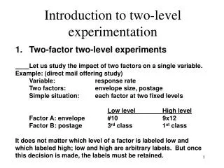
Introduction to two-level experimentation. 1. Two-factor two-level experiments Let us study the impact of two factors on a single variable. Example: (direct mail offering study) Variable: response rate Two factors: envelope size, postage Simple situation: each factor at two fixed levels

E N D
Introduction to two-level experimentation 1. Two-factor two-level experiments Let us study the impact of two factors on a single variable. Example: (direct mail offering study) Variable: response rate Two factors: envelope size, postage Simple situation: each factor at two fixed levels Low level High level Factor A: envelope #10 9x12 Factor B: postage 3rd class 1st class It does not matter which level of a factor is labeled low and which labeled high; low and high are arbitrary labels. But once this decision is made, the labels must be retained.
There are four possible experimental combinations. These are called treatments, or treatment combinations: • a0b0 A at low level, B at low level a0b1 A at low level, B at high level a1bo A at high level, B at low level a1b1 A at high level, B at high level
For now we will imagine that each of the four treatments is run once; the experiment will be called a two-factor two-level factorial design (without replication). For each treatment the response rate is computed. The four observed response rates are called yields or responses. The symbols used for treatments are also used for yields (or yield means for with replications case). Thus, a0b0also represents the yield when the treatment a0b0 is run.
2. Estimating effects in two-factor two-level experiments Estimate of the effect of A a1b1 - a0b1 estimate of effect of A at high B a1b0 - a0b0 estimate of effect of A at low B sum/2 estimate of effect of A over all B Estimate of the effect of B a1b1 - a1b0 estimate of effect of B at high A a0b1 - a0b0 estimate of effect of B at low A sum/2 estimate of effect of B over all A
Estimate the interaction of A and B a1b1 - a0b1 estimate of effect of A at high B a1b0 - a0b0 estimate of effect of A at low B difference/2 estimate of the effect of B on the effect of A Called the interaction of A and B a1b1 - a1b0 estimate of effect of B at high A a0b1 - a0b0 estimate of effect of B at low A difference/2 estimate of the effect of A on the effect of B Called the interaction of B and A
Note that the two differences in the interaction estimate are identical; by definition, the interaction of A and B is the same as the interaction of B and A. In a given experiment one of the two literary statements of interaction may bepreferred by the experimenterto the other; but both have the same numerical value.
3. Remarks on effects and estimates General remarks Note the use of all four yields in the estimate of the effect of A, the effect of B, and the effect of the interaction of A and B; all four yields are needed and are used in each estimate. Note also that the effects of each of the factors and their interaction can be and are assessed separately,this in an experiment in which both factors vary simultaneously. Note that, with respect to the two factors studied, the factors themselves together with their interaction are, logically, all that can be studied. These are among the merits of these factorial designs.
Remarks on interaction Many people feel the need for experiments which will reveal the effect, on the variable under study, of factors acting jointly. This is what we have called interaction. The simple experimental design discussed here provides a way of estimating such interaction, with the latter defined in a way which corresponds to what many scientists and managers have in mind when they think of interaction. It is useful to note that interaction was not invented by statisticians. It is a joint effect existing, often prominently, in the real world. Statisticians have (wonderfully enough!!) provided ways and means to measure it.
4. Symbolism and language A is called a main effect. Our estimate of A is often simply written A. B is called a main effect. Our estimate of B is often simply written B. AB is called an interaction effect. Our estimate of AB is often simply written AB. So the same letter is used, generally without confusion, to describe the factor, to describe its effect, and to describe our estimate of its effect. Keep in mind that it is only for economy in speaking and writing that we sometimes speak/write about an “effect” rather than an “estimate of the effect." We should always remember that all quantities formed from the yields are, OF COURSE, estimates.
A B AB a0b0 - - + a0b1 - + - a1b0 + - - a1b1 + + + 5. Table of signs The following table is useful: Notice than in estimating A, the two treatments with A at high level are compared to the two treatments with A at low level. Similarly B. This is, of course, logical. Note also that the signs of treatments in the estimate of AB are the products of the signs of the corresponding treatments of A and B. Note, finally, that in each estimate, plus and minus signs are equal in number. Effect = Ave of “+” – Ave of “-”.
B low high Example 1 B low high Example 2 10 15 15 15 10 12 13 15 low high low high A A B low high Example 4 Example 3 B low high 12 12 12 12 10 13 13 10 low high low high A A 6 ? A B AB 1 3 2 0 2 2.5 2.5 -2.5 3 0 0 -3 4 0 0 0 Discussion of examples: Notice that in Examples 2 & 3 interaction is as large as or larger than main effects.
Change of scale, by multiplying each yield by a constant (3 inches 3x2.54 cm), multiplies each estimate by the constant but does not affect the relationship of estimates to each other. Addition of a constant to each yield does not affect the estimates. The numerical magnitude of estimates is not important here; it is their relationship to each other.
1 a b ab -1 -1 1 1 -1 -1 -1 1 -1 1 1 1 A = (-1+a-b+ab)/2 B = (-1-a+b+ab)/2 AB = (1-a-b+ab)/2 Earlier we formed: estimate of 2A estimate of 2B estimate of 2AB
Which for present purposes we replace by: 1 a b ab Z . . . . . . . . 1 2 1 2 1 2 1 2 1 2 1 2 1 2 1 2 1 2 - 1 2 1 2 1 2 - A - - B - - AB Now we can see that these coefficients of the three contrasts are orthogonal and thus A, B and AB constitute orthogonal estimates and their SS’s can be found accordingly. (For example, SSA = RxZA^2.)
8. Three factors each at two levels The dependent variable is response rate of a direct mail offering. lowhigh A postage 3rd class 1st class B price $9.95 $12.95 C envelope size #10 9 x 12 Treatments (also yields) (a) old notation (b) new notation. (a) a0b0c0 a0b0c1 a0b1c0 a0b1c1 a1b0c0 a1b0c1 a1b1c0 a1b1c1 (b) 1 c b bc a ac ab abc Yates (standard) order : (add factors one after one) 1 a b ab c ac bc abc
9. Estimating effects in three-factor two-level designs Estimate of A (1) a - 1 estimate of A, with B low and C low (2) ab - b estimate of A, with B high and C low (3) ac - c estimate of A, with B low and C high (4) abc - bc estimate of A, with B high and C high = (a+ab+ac+abc-1-b-c-bc)/4, = (-1+a-b+ab-c+ac-bc+abc)/4, (in Yates’ order)
Estimate of AB (the effect of B on the effect of A) effect of A with B high - effect of A with B low, all at C high plus effect of A with B high - effect of A with B low, all at C low Note that interaction are averages. Just as our estimate of A is an average of response to A over all B and all C, so our estimate of AB is an average response to AB over all C. AB = {[(4)-(3)] + [(2) - (1)]}/4 = {1-a-b+ab+c-ac-bc+abc)/4, in Yates’ order.
Estimate of ABC (the effect of C on AB) interaction of A and B, at C high minus interaction of A and B at C low ABC = {[(4) - (3)] - [(2) - (1)]}/4 = (-1+a+b-ab+c-ac-bc+abc)/4, in Yates’ order.
This is our first encounter with a three-factor interaction. It measures the impact on the response rate of interaction AB as C (envelope size) goes from #10 to 9 x 12. Or, it measures the impact on response rate of interaction AC as B (price) goes from $9.95 to $12.95. Or, finally, it measures the impact on the response rate of interaction BC as A (postage) goes from 3rd class to 1st class. As with two-factor two-level factorial designs, the formation of estimates in three-factor two-level factorial designs can be summarized in a table:
A B AB C AC BC ABC 1 - - + - + + - a + - - - - + + b - + - - + - + ab + + + - - - - c - - + + - - + ac + - - + + - - bc - + - + - + - abc + + + + + + + Plus-Minus Table
10. DATA ANALYSIS 1 a b ab c ac bc abc .062 .074 .010 .020 .057 .082 .024 .027 A = main effect of postage = .0125 B = main effect of price = -.0485 AB = interaction of A and B = -.0060 C = main effect of envelope size = .0060 AC = interaction of A and C = .0015 BC = interaction of B and C = .0045 ABC = interaction of A, B, and C = -.0050 NOTE: ac = largest yield; AC = smallest effect.
We describe several of these estimates, though on later analysis of this example, taking into account the unreliability of estimates based on a small number (eight) of data values, some estimates may turn out to be so small in magnitude as not to reject the null hypothesis that the corresponding true effect is zero. The largest estimate is -.0485, the estimate of B; an increase in price, from $9.95 to $12.95, is associated with a decline in response rate. The interaction AB = -.0060; an increase in price from $9.95 to $12.95 reduces the effect of A, whatever it is (A = .0125), on response rate. Or equivalently,
an increase in postage from 3rd class to 1st class reduces (makes more negative) the already negative effect (B = -.0485) of price. Finally, ABC = -.0050. Going from #10 to 9 x 12 envelope, the negative interaction effect AB on response rate becomes even more negative. Or, going from low to high price, the positive interaction effect AC is reduced. Or, going from low to high postage, the positive interaction effect (BC) is reduced. All three descriptions of ABC have the same numerical value, but the direct marketer would select one of them, and then say it better!
11. Number and kinds of effects We introduce the notation 2k. This means a k-factor design with each factor at two levels. The number of treatments in an unreplicated 2k design is 2k. The following table shows the number of each kind of effect for each of the six two-level designs shown across the top.
22 23 24 25 26 27 2 3 4 5 6 7 1 3 6 10 15 21 1 4 10 20 35 1 5 15 35 1 6 21 1 7 1 main effect 2 factor interaction 3 factor interaction 4 factor interaction 5 factor interaction 6 factor interaction 7 factor interaction 3 7 15 31 63 127 In a 2k design the number of r-factor effects is Ck = k!/[r!(k - r)!] r
Notice that the total number of effects estimated in any design is always one fewer than the number of treatments: One need not repeat the earlier logic to determine the forms of estimates in 2k designs for higher values of k. A table going up to 25 is on P.265, Table 9.4. in a 22 design there are 22=4 treatments; we estimate 22-1=3 effects, in a 23 design there are 23=8 treatments; we estimate 23-1=7 effects.
Exercise: Write down the plus-minus table for the 24 design.
Note: for2k designs with replications All terms (1, a, b, …) are “treatment combinations” or “yield means of the treatment combinations”. In the previous example, yields are response rates and thus (1, a, b, …) are average response rates for the corresponding treatment combinations.
12. Yates’ forward algorithm 1. Applied to Complete Factorials (Yates, 1937) A systematic method of calculating estimates of effects. For complete factorials first arrange the yields in Yates’ (standard) order. Addition, then subtraction of adjacent yields. The addition and subtraction operations are repeated until 2k terms appear in each line: for a 2k there will be k columns of calculations.
Example: 23 Yield 1st. Column 2nd. Column 3rd. Column 1 a b ab c ac bc abc a+1 ab+b ac+c abc+bc a-1 ab - b ac - c abc -bc ab+b +a+1 abc+bc+ac+ c ab-b+a-1 abc-bc+ ac- c ab+b-a-1 abc+bc- ac-c ab-b-a + 1 abc-bc-ac+ c abc+ bc+ac+ c+ab +b+a+1 abc - bc+ac - c+ab - b+a -1 abc+ bc- ac - c+ab+ b -a -1 abc - bc- ac+ c+ab - b -a+1 abc+ bc+ac+ c -ab - b -a-1 abc - bc+ac - c-ab+ b -a+1 abc+ bc- ac - c-ab- b+a+1 abc - bc- ac+ c-ab+ b+a-1 Checking in our 23 table of signs, entries in the third column estimate, respectively, (=1) A B AB C AC BC ABC Note the line-by-line correspondence between yields (lower case letters in the left column of the table) and factors estimated (upper case letters directly above). Treatments and estimates of effects are in Yates’ order.
Yates’ Forward Algorithm EXAMPLE: 23 already used. Tr. Yield 1stCol 2ndCol 3rdCol 1 .062 .136 .166 .356 - a .074 .030 .190 .050 estimate of 4A b .010 .139 .022 -.194 estimate of 4B ab .020 .051 .028 -.024 estimate of 4AB c .057 .012 -.106 .024 estimate of 4C ac .082 .010 -.088 .006 estimate of 4AC bc .024 .025 -.002 .018 estimate of 4BC abc .027 .003 -.022 -.020 estimate of 4ABC Again, note the line-by-line correspondence between treatments and estimates; both are in Yates’ order.
13. Main effects in the face of large interactions Several writers have cautioned against making statements about main effects when the corresponding interactions are large; interactions describe the dependence of the impact of one factor on the level of another; in the presence of large interaction, main effects may not be meaningful.
EXAMPLE Yields are purchase intent for cigarettes. low levelhigh level Sex Male Female Brand Frontiersman April The yields are 1 = 4.44 s = 2.04 b = 3.50 sb = 4.52 The estimates are S = -.69 B = +.77 NP = +1.71. In the face of such high interaction we now specialize the main effect of each factor to particular levels of the other factor. Effect of B at high level S = sb - s = 4.52 - 2.04 = 2.48 Effect of B at low level S = b - 1 = 3.50 - 4.44 = -.94, which appear to be more valuable for branding strategy than the mean (.77) of such disparate numbers.
Note that answers to these specialized questions are based on fewer than 2k yields. In our numerical example, with interaction SB prominent, we have only two of the four yields in our estimate of B at each level of S. In general we accept high interactions wherever found and seek to explain them; in the process of explanation, main effects (and lower-order interactions) may have to be replaced in our interest by more meaningful specialized effects.
14. Levels of factors The responses or yields are conjectured to follow the curves Yield p1 58 47 p2 30 29 22 20 18 15 Temperature t1 t2 t3 t4 Compare P effect at (t1, t2) vs (t3, t4) or others.
at (t1, t2): P= -8-29 = -18.5 T= (29-22)+(58-30) = +17.5 PT=-29-(-8) = 7-28 = -10.5 P= 27+3 = 15 T= (18-47)+(15-20) = -17 PT= 3-27 = -29-(-5) = -12 2 2 2 2 2 2 2 2 AtP effect (P2-P1) t1 22 - 30 = -8 t2 29 - 58 = -29 t3 47 - 20 = +27 t4 18 - 15 = +3 at (t3, t4): at (t1, t3) ?
It is only when the conjectured responses in the diagram are in fact linear and parallel that choice of levels is unimportant. One must acknowledge the essentially circular nature of the discussion. One needs to have a good idea of the response curves in order to fix the levels of an experiment which seeks essentially to discover the response curves. But this kind of circularity characterizes all experimental science.
15. Factorial designs vs. designs varying one factor at a time Example: Variable: Profitability Two factors each at two levels: Time Frame: Past Year Future Mode: Numerical Non-numerical Vary one factor at a time. Hold Time Frame at past year and take two observations on profitability at each mode; we take two observations to facilitate comparison with a factorial design. Then we take two more observations at (Numerical, Future):
Mode Non-N. Num. Time Frame Past Future
Now consider an unreplicated 22 factorial design. Mode Non-N. Num. Time Frame Past Future
Comparison of the 22 factorial design and the one-factor-at-a-time design: In the factorial design each estimate of a main effect is based on all four yields. Each estimate has as much supporting data (is as reliable) as the corresponding estimate from the more costly six-yield one-factor-at-a-time design; the latter was able to use only four of its six yields in each estimate. In the factorial design, interaction = (whatever it is), an effect not estimable from the one-factor-at- a-time design. a. b.
In the factorial design, each main effect is estimated over both levels of the other factor, not at one level as in the case of the one-factor-at-a-time design; this increased generality is usually, though, not always, attractive. If interaction is high, we may, as we have seen, want the effect of each factor at each level of the other factor; this the one-factor-at-a-time design can provide at two points (the Time Frame effect at Num. and the Mode effect at Past ) better than the factorial design. But the one-factor-at-a-time design will not reveal the magnitude of interaction in the first place!! c.
An estimate of the effect of factors other than the two factors studied is possible in the 6-yield experiment. Thus, the differences in yields at a given treatment combination cannot be due to Time Frame, Mode, or their interaction since Time Frame and Mode were fixed throughout each difference. These differences must be due to other factors. However, a replicated factorial experiment can, of course, provide such an estimate. d.
f. One-factor-at-a-time designs are less vulnerable to missing yields. The general judgment, particularly in recent years, is that factorial designs are definitely superior to one-factor-at-a-time experimentation.
Another Example In a complete 25 design, we have 32 treatment combinations and, without replication, 32 data values. Each data value contributes to the estimate of each Effect. Thus, each Effect has the “reliability” of 32 data values. To achieve the same reliability doing “one-at-a-time” experimentation, we would need 96 (NINETY-SIX!) data values:
AL, BL, CL, DL, EL AH, BL, CL, DL, EL AL, BH, CL, DL, EL AL, BL, CH, DL, EL AL, BL, CL, DH, EL AL, BL, CL, DL, EH A B C D E Having 16 of each of these 6 treatment combinations ( = 96 data values in total) would give us estimates of each main Effect with the same “reliability” of 32 data values. BUT, WHAT ABOUT INFORMING US ABOUT THE PRESENCE OF INTERACTIONS??
16. Factors not studied In any experiment factors other than those studied may be influential. Their presence is sometimes acknowledged under the title “error.” They may be neglected, but the cost of neglect could be high. It is important to deal explicitly with them; even more, it is important to measure their impact. How?