Download
1 / 151
1.51k likes | 1.67k Views
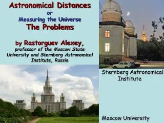
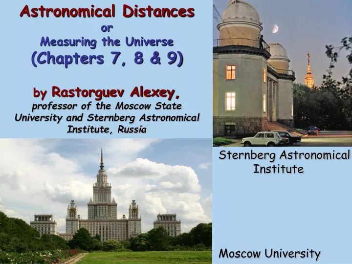
Astronomical Distances or Measuring the Universe (Chapters 7, 8 & 9) by Rastorguev Alexey, professor of the Moscow State University and Sternberg Astronomical Institute, Russia. Sternberg Astronomical Institute Moscow University. Content.

E N D
Astronomical Distancesor Measuring the Universe(Chapters 7, 8 & 9)by Rastorguev Alexey,professor of the Moscow State University and Sternberg Astronomical Institute, Russia Sternberg Astronomical Institute Moscow University
Content • Chapter Seven: BBW: Moving Photospheres (Baade-Becker-Wesselink technique) • Chapter Eight: Cepheid parallaxes and Period – Luminosity relations • Chapter Nine: RR Lyrae distance scale
Chapter Seven BBW: Moving Photospheres (Baade-Becker-Wesselink technique)
Astronomical Background • W.Baade-W.Becker-A.Wesselink-L.Balona technique (BBWB) is applicable to pulsating stars (Cepheids and RR Lyrae variables) or stars with expanding envelopes (SuperNovae) • W.Baade (Mittel.Hamburg.Sternw. V.6, P.85, 1931); W.Becker (ZAph V.19, P.289, 1940); A.Wesselink (Bull.Astr.Inst.Netherl. V.10, P.468, 1946): • photometry and radial velocities give rise to radius measurement and independent calculation of star’s luminosity
(a) For a pair of phases with the same temperature and color (say, B-V), the Cepheid’s apparent magnitudes V differ due only to the ratio of stellar radii: (b) Radii difference (R1-R2) can be calculated by integrating the radial velocity curve, due to VR ~ dR/dt R1 R2 B-V Pulsation Phase
A number of pairs • (R1 – R2) ~∫VR·dt and R1/R2 ≈ 10-0.2m give rise to the calculation of mean radius, <R> = (Rmax + Rmin)/2
I. BBW Surface-brightness technique (SB) θLD Eλ • θLD is “limb-darkened” angular diameter • Flux incident, Eλ ~ Φλ·θLD2, where Φλ being surface brightness (do not depending on the star’s distance!) • Apparent magnitude, mλ ~ -2.5 log Eλ, so • 0.5∙log θLD ~ -0.1·mλ - Fλ + c , with Fλas the “surface-brightness parameter”
It can be easily shown that the “surface-brightness parameter” is expressed as • Fλ = 4.2207 – 0.1∙mλ0 - 0.5∙ log θLD = =log Teff + 0.1 BC(λ), • where BC(λ) is the bolometric correction to the mλ magnitude, i.e. • BC(mλ) = Mbol - Mλ
The surface-brightness parameter is shown to relate with the color CI (due to surface brightness dependence on the effective temperature Φλ ~ Teff4 and CI-Teff relations) • Fλ≈a·CIλ + b • Example relation is shown; interferometric calibrations (Nordgren et al. AJ V.123, P.3380, 2002)
The calibrations for surface brightness parameter, Fλ, can be also derived from the photometric data for normal stars (dwarfs, giants and supergiants) with the distances determined, say, by precise trigonometric technique or other data • See, for example, M.Groenewegen “Improved Baade-Wesselink surface brightness relations” (MNRAS V.353, P.903, 2004)
From both relations, • 0.5∙log θLD ≈ -0.1·mλ - Fλ + c • Fλ≈a·CIλ+ b • log θLD ~ -0.2·mλ + 2a·CIλ + const • Direct calculation of star’s angular diameter vs time Light-curve Color-curve
Radial velocity curve integration gives absolute radius change, and being relate to apparent angular diameter change, distance to the pulsating star follows
II. Maximum Likelyhood technique by L.Balona(MNRAS V.178, P.231-243,1977) uses all light curve and precise radial velocity curve • Background: • (a) Stefan-Boltzmann low: Lbol ~ σT4 • (b) Effective temperature and bolometric correction are connected with normal color (see examples) • (c) Radius change comes from the integration of the radial velocity curve
Luminosity classes: Working interval lg Teff – (B-V)0relation by P.Flower (1996)
Working interval Luminosity classes ΔMbol ΔMbol – (B-V)0relation by P.Flower (ApJ, V469, P.355, 1996)
Quadratic approximations can be written forlgTeff,ΔMbolby(B-V)0(and by other normal colors) in the range0.2 < (B-V)0 < 1.6
Here constantsA, BandC: These constants enclose information on color excess E(B-V) and the star’s distance d
How to calculate the radius change? Moving photosphere dS: ring area Contribution of the circular ring to the observed radial velocity -V0: photosphere velocity (to the observer)
CalculatingR(t)=<R>+r(t):integrating radial velocity curveVrRing contribution to the measured radial velocity:
Mean radial velocity weighted along star’s limb = observed Vr pis the projection factor connecting radial velocity and the photosphere speed
Projection factor values: • In the absence of limb darkeningp=3/2 • In most studiesp=1.31 accepted • But: projection factor depend on • Limb darkening coefficient • Velocity of the photosphere • Instrumental line profile used to measure radial velocity
Theoretical spectral line will be distorted due to instrumental profile
Line profile calculation enables to derive theoretical value of the projection factor,pObserved line profile (with taking into account line broadening due to instrumental effects) can be calculated as the convolution
Some examples of the line profiles for different line broadening due to instrumental effects Instrumental width Theoretical profile Solid: normal Observed profile Small velocity Good Gaussian fit
Some examples of the line profiles for different line broadening due to instrumental effects Instrumental width Theoretical profile Normal curve Observed profile Large velocity Normal curve (blue line) Bad Gaussian fit
Modern calculations confirm the variation of p by at least ~5-7% due to different effects • (Nardetto et al., 2004; Groenewegen, 2007; Rastorguev & Fokin, 2009)
Example: projection factor and line width vs photosphere velocity, V0 From Gauss tip From line tip
Projection factor p and its variation with the velocity V0 , limb darkening coefficient ε and instrumental width σ should be “adjusted” to proper spectroscopic technique used for radial velocity measurements • Example: More than 20000 VR measurements have been performed by Moscow team for ~165 northern Cepheids with characteristic accuracy ~0.5 km/s and σ ~ 15 km/s
Radius change, r(t), can be calculated by integrating the radial-velocity curve, Vr (t), from some t=0 (where R(0)=<R>)
Example:TT Aql radial velocity curve (upper panel) and radius change (bottom panel) Vr, km/s ΔR, Solar units Pulsation phase
Fitting the light curve for TT Aql Cepheid (+) with the model (solid line) V Pulsation phase
Steps to luminosity calibration • <R>, A, B, C enable: • To calculate mean bolometric and visual luminosity of the star and its distance • To refine transformations of Teff to normal colors and bolometric corrections (additionally) • BBWB technique has been applied to Cepheid and RR Lyrae variables and turned out to be very effective and independent tool for P-L calibrations (see later)
For Fundamental tone Cepheids: • log R/RSun = 1.23 (±0.03) + (0.62 ±0.03) log P by M.Sachkov (2005) Cepheid radii can be used to classi- fy Cepheids by the pulsation mode (first-over- tone pulsators have shorter peri- ods at equal radii) FU 1st
Well known possibility to measure the distances to some SuperNova remnants via their angular sizes and the envelope expansion velocities is also can be considered as the modification of the moving photospheres technique • Possible explosion asymmetry can induce large errors to estimated parameters
t1 SN t2 VR D Δφ
Optical and NIR interferometric direct observations of the radii changes of nearest Cepheid are of great importance and very promising tool to measure their distances and correct the distance scale
B.Lane et al. (ApJ V.573, P.330, 2002): • Palomar PTI 85-m base length optical interferometer Distance within 10% error Phase
P.Kervella et al. (ApJ V.604, L113, 2004): interferometric (ESO VLT) apparent diameter measurements (filled circles) as compared to BW SB technique (crosses) D ~ 566 ±20 pc Very good agreement
Chapter Eight Cepheid parallaxes and Period – Luminosity relations • Astrophysical background • Overtone pulsators • Use of Wesenheit index • Luminosity calibrations • P-L or P-L-C ?
Cepheids “econiche” Cepheids as calibrators for these methods 100 pc … 50 Mpc pc
Cepheids and RR Lyrae variable stars populate Instability Strip on the HRD (see blue strip) where most stars become unstable with respect to radial pulsations • Instability Strip crosses all branches, from supergiants to white dwarfs
G.Tammann et al. (A&A V.404, P.423, 2003) • Instability strip for galactic Cepheids (members of open clusters and with BBWB radii) in more details: • MV-(B-V) and MI-(V-I) CMDs
Comprehensive review of the problem by: Alan Sandage & Gustav Tammann “Absolute magnitude calibrations of Populations I and II Cepheids and Other Pulsating Variables in the Instability Strip of the Hertzsprung-Russell Diagram” (ARAA V.44, P.93-140, 2006)
Cepheids: named after δCepheus star, the first recognized star of this class • Young (< 100 Myr) and massive (3-8 MSun) bright (MV up to -7m) radially pulsating variable stars with strongly regular brightness change (light curves) • Typical Periods of the pulsations: from ~1-3 to ~100 days (follow from P ~ (Gρ)-1/2 expression for free oscillations of the gaseous sphere: mean mass density of huge supergiants, ρ, is very small as compared to the Sun)
Evolution tracks for 1-25MSun stars on the HRD • Luminosities: from ~100 to 30 000 that of the Sun • Evolution status: yellow and red supergiants, fast evolution to/from red (super)giants while crossing the instability strip (solid lines)
Relative fraction of Cepheids population depends on the evolution rate while crossing the instability strip: • slower evolution means more stars at the appropriate stage
The differences in the evolution rates at different crossings give rise to the questions on the relative contribution of bright and faint Cepeids for the same period value Cepheids evolution tracks, the instability strip and P=const lines (red) lg L • (a) Tracks are not parallel to the lines of constant periods • Evolutional period change happens • (b) Evolution rate during 2nd & 3rd crossings is slower than for 1st crossing, defining the IS population fraction • (c) Luminosity depend on the crossing number IS An extra source of P-L scatter
dP/dt is visible when observing on long time interval (~100 yr)