Download
1 / 26
260 likes | 416 Views
Recursion. Breaking down problems into solvable subproblems Chapter 7. The good and the bad. Pluses Code easy to understand May give different view of problem Sometimes, efficient Bad overhead of functions calls (20-30%) may be hard to analyze cost not apparent

E N D
Recursion Breaking down problems into solvable subproblems Chapter 7
The good and the bad • Pluses • Code easy to understand • May give different view of problem • Sometimes, efficient • Bad • overhead of functions calls (20-30%) • may be hard to analyze • cost not apparent • can be very inefficient: exponential worse!
Finite Induction • Finite Induction principle • Let Sn be a proposition depending on n • Base Case: Show that S1 is true • Inductive case: • Assume Sk and prove Sk+1 • Conclude: Sn is true for all n >= 1. • Variant: • Base Case: Show that S1 is true • Inductive case: • Assume S1,S2 … Sk and prove Sk+1 • Conclude: Sn is true for all n >= 1.
Example • Proofs involve two tricks • recognize subproblem (make take rearranging) • follow your nose • Sn: 1+2…+n = n(n+1)/2 • Base case: S1 is true 1 = 1(1+1)/2 check • Inductive Case • Given Sk, show Sk+1, i.e. 1+2+…k+1 = something. • 1+2..+k+ k+1 = k(k+1)/2 + k+1 = (k*k+k+ 2k+2)/2 = (k+1)(k+2)/2. QED.
Example: Complete k-ary tree • Sn: A full m-ary tree of depth n has (m n+1-1)/(m-1) nodes • S0: (m1 -1)/(m-1) = 1 . • Assume Sk (visualize it) m m^2 … m^k at depth k ... ...
The Math • Visualization provides the recurrence Nodes in a Sk+1 trees is # in Sk tree + m*number of leaves in Sk = (mk+1-1)/(m-1) +m*mk = (mk+1-1)/(m-1) + m^(k+2)/(m-1) -m^(k+1)/(m-1) = (m^(k+2) -1)/(m-1)
Fibonacci • Fib(n) if (n <= 1) return 1 else return fib(n-1)+ fib(n-2) • What is the cost? • Let c(n) be number of calls • Note c(n) =c(n-1)+c(n-2)+1 >= 2*c(n-2) • therefore c(n) >= 2n/2*c(1), ie. EXPONENTIAL • Also c(n)<= 2*c(n-1) so • c(n) <= 2n*c(1). • This bounds growth rate. • Is 3n in O(2n)?
Dynamic Fibonacci • Recursion Fibonacci is bad • Special fix • Compute fib(1), fib(2)….up to fib(n) • Reordering computation so subproblems computed and stored: example of dynamic programming. • Easiest approach: use array • fib(n) • array[1] =array[2]=1 • for i = 3…n • array[i] = array[i-1]+array[i-2] • return array[n] • note: you don’t need an array. • This works for functions dependent on lesser values.
Combinations (k of n) • How many different groups of size k and you form from n elements. • Ans: n!/[(n-k)! * k!] • Why? # of permutations of n people is n! # of permutations of those invited is k! # of permutations of those not invited is (n-k)! • Compute it. DOES not compute! • Dynamic does. • Note: C(k,n) = C(k-1,n-1) +C(k,n-1) • C(0,n) = 1 • Use a 2-dim array. That’s dynamic programming
General Approach (caching) • Recursion + hashing to store solution of subproblems • Idea: • fib(n) • if (in hash table problem fib(n)) return value • else fib(n) = fib(n-1) + fib(n-2). • How many calls will there be? • How many distinct subproblems are there. • Good: • don’t need to compute unneeded subproblems • simpler to understand • Bad: overhead of hashing • Not needed here, since subproblems obvious.
Recursive Binary Search • Suppose T is a sorted binary tree • values stored at nodes • Node • node less, more • int key • Object value • Object find(int k) // assume k is in tree • if ( k == key) return value; • else if (k < key) return less.find(k) • else if (k >key) return more.find(k) • What is the running time of this?
Analysis • If maximum depth of tree is d, then O(d). • What is maximum depth? • Worst case: n • What does tree look like? • Best case: log(n) • What will tree look like. • So analysis tells us what we should achieve, i.e. a balanced tree. It doesn’t tell us how. • Chapter 18 shows us how to create balanced trees.
Binary Search • Solving f(x) = 0 where a<b, f(a)<0, f(b)>0 • Solve( f, a, b) (abstract algorithm) • mid = (a+b)/2 • if -epsilon< f(mid) < epsilon return mid (*) • else if f(mid) <0 return f(mid,b); • else return f(a,mid) • Note: epsilon is very small; real numbers are not dealt with exactly by computers • Analysis: • Each call divides the domain in half. • Max calls is number of bits for real number • Note algorithm may not work on real computer -- this depends on how fast f changes.
Divide and Conquer: Merge Sort • Let A be array of integers of length n • define Sort (A)recursively via auxSort(A,0,N) where • Define array[] Sort(A,low, high) • if (low == high) return • Else • mid = (low+high)/2 • temp1 = sort(A,low,mid) • temp2 = sort(A,mid,high) • temp3 = merge(temp1,temp2)
Merge • Int[] Merge(int[] temp1, int[] temp2) • int[] temp = new int[ temp1.length+temp2.length] • int i,j,k • repeat • if (temp1[i]<temp2[j]) temp[k++]=temp[i++] • else temp[k++] = temp[j++] • for all appropriate i, j. • Analysis of Merge: • time: O( temp1.length+temp2.length) • memory: O(temp1.length+temp2.length)
Analysis of Merge Sort • Time • Let N be number of elements • Number of levels is O(logN) • At each level, O(N) work • Total is O(N*logN) • This is best possible for sorting. • Space • At each level, O(N) temporary space • Space can be freed, but calls to new costly • Needs O(N) space • Bad - better to have an in place sort • Quick Sort (chapter 8) is the sort of choice.
General Recurrences • Suppose T(N) satisfies • Assume N is a power of 2 (wlog) • T(N) = 2T(N/2)+N • T(1) = 1 • Then T(N) = NLogN+N or T is O(NlogN) • Proof • T(N)/N = T(N/2)/(N/2) +1 • T(N/2)/ (N/2) = T(N/4)/ (N/4) + 1 etc. • … • T(2)/2 = T(1)/1 + 1
Telescoping Sum • Sum up all the equations and subtract like terms: • T(N)/N = T(1)/1+ 1*(number of equations) • Therefore T(N) = N +N*logN or O(N*log(N)) • Note: The same proof shows that the recurrence • S(N) = 2*S(N/2) is O(N). • What happens if the recurrence is T(N) =2*T(N/2)+k? • What happens if the recurrence is T(N)=3*T(N/3)..? • General formula
General Recurrence Formulas • Suppose • Divide into A subproblems • Each of relative size B (problem size/subproblem size) • k overhead is const*Nk • Then • if A>Bk T(N) is O(NlogB(A)) • if A= Bk T(N) is O(NklogN) • if A<Bk T(N) is O(Nk) • Proof: telescoping sum, see text. • Example: MergeSort; A=2, B=2, k = 1 (balanced) • MergeSort is O(NlogN) as before.
Dynamic Programming • Smith-Waterman Algorithm has many variants • Global SW algorithm finds the similarity between two strings. • Goal: given costs for deleting and changing a character, determine the similarity of two strings. • Main application: given two proteins (sequence of amino acids), how far apart are they? • Evolutionary trees • similar sequences define proteins with similar functions • can compare across species • other version deal with finding prototype/consensus for family of sequences
Smith - Waterman Example • See Handout from Biological Sequence Analysis • In this example, A,R,…V are the 20 amino acids • Fig 2.2 defines how similar various amino acids are to one another • Fig 2.5 shows the computation of the similarity of two sequences • The deletion cost is 8. • The bottom right hand corner gives the value of the similarity • Tracing backwards computes the alignment.
SW subproblem merging c(i-1,j-1) c(i-1,j) c(i,j-1) c(i,j) Down: extend matching by deleting char si Right: extend match by deleting char tj Diagonal: extend match by substitution, if necessary
Smith-Waterman Algorithm • Recursive definition: -- find the subproblems • Let s and t be the strings of lengths n and m. • Define f(i,j) as max similarity score of matching the initial i characters of s with initial j characters of t. • f(0,0) = 0 • For i>0 or j>0 • let sim(si,tj) be similarity of char si and char tj. • Let d be cost of deletion. • f(i,j) = max {f(i-1,j) -d, f(i,j-1)-d, f(i-1,j-1) +sim(si,tj)} • Analysis: O(n*m)
Matrix Review • A matrix is 2-dim array of number, e.g. Int[2][3] • Matrices represent linear transformations • Every linear transformation is a matrix product of scale changes and rotations • The determinant of a matrix is the change in volume of the unit cube. • Matrices are used for data analysis and graphics • If M1 has r1 rows and c1 columns and • M2 has r2 rows and c2 columns, and r2= c1 • then M3 = M1*M2 has r1 rows and c2 columns where • M3[i][j]= (row i of M1) * (col j of M2) (dot product) • In general M1*M2 =/= M2*M1 (not commutative) • but (M1*M2)*M3 = M1*(M2*M3) (associative)
Multiplying Many Matrices • Let Mi i=1..n be matrices with ri-1 rows and ri columns • How many ways to multiply M1*M2…M*n? • exponential (involves Catalan numbers) • But O(N3) dynamic programming algorithm! • Let mij = min cost of multiplying Mi*….*Mj • Subproblem Idea: Mi*… *Mk * M k+1*…*Mj • if i = j then mij = 0 • if j>i then mij = min{ i<=k <j: mik + mk+1,j+ ri-1rkrj} • Cost of this step is O(N). • To fill in all mij (i<j) yields O(N3) algorithm
Summary • Recursion begat divide and conquer and dynamic programming • General Flow • Subdivide problem • Store subsolutions • Merge subsolutions • Beware of the costs: • cost of subdivision • cost of storage • cost of combining subsolution • Can be very effective