Download
1 / 41
810 likes | 2.53k Views
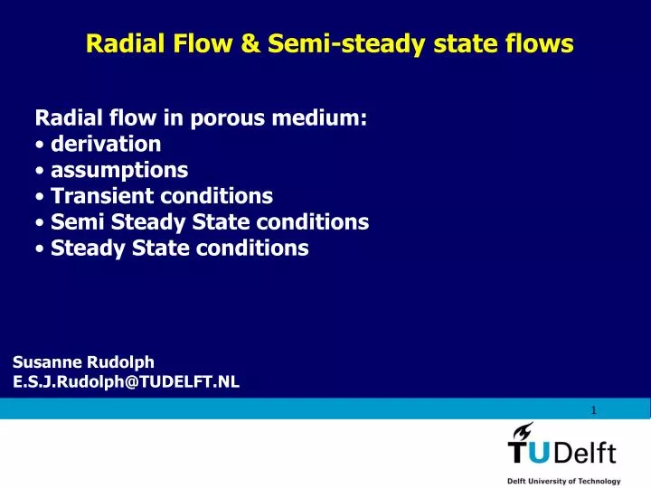
Radial Flow & Semi-steady state flows . Radial flow in porous medium: derivation assumptions Transient conditions Semi Steady State conditions Steady State conditions. Susanne Rudolph E.S.J.Rudolph@TUDELFT.NL. Recap of last classes (general).

E N D
Radial Flow & Semi-steady state flows • Radial flow in porous medium: • derivation • assumptions • Transient conditions • Semi Steady State conditions • Steady State conditions Susanne Rudolph E.S.J.Rudolph@TUDELFT.NL
Recap of last classes (general) In last classes you got accustomed with Darcy’s law to describe one-phase flow through porous medium. Darcy’s law needs to be combined to mass balance to allow calculation of flow through porous medium. So far, only description of flow at low Reynolds numbers (laminar flow), steady-state and for incompressible fluids and rock. Equations for linear and radial flow have been derived.
What will be done next? General equation will be derived to describe the flow through porous medium – in cartesian and radial coordinates. Discussion of staedy state, semi-steady state and transition conditions. General description of steady state, semi-steady state and transition conditions. Detailed description of transient conditions.
Derivation of radial flow equation in porous medium Derivation in radial form to allow description of flow in porous medium close to a well. Equations in radial form create ‘feeling’ for flow through porous medium. Cartesian form commonly used in reservoir simulations.
Derivation of radial flow equation in porous medium Assumptions: Reservoir is homgenous in all rock properties. Isotropic behavior of permeability. Production well is completed over the whole formation thickness -> radial flow can be assumed. Formation is fully saturated by a single fluid.
Derivation of radial flow equation in porous medium Radial cell geometry Volume element for mass balance (accounting for porosity): dV = 2..r.h..r
Derivation of radial flow equation in porous medium Mass balance: Mass flow rate (in) – mass flow rate (out) = rate of change of mass in volume element The left hand of the equation can be rewritten by:
Derivation of radial flow equation in porous medium With this the mass balance simplifies to: Darcy’s law for radial, horizontal flow is: Substituting this into the mass balance results in:
Derivation of radial flow equation in porous medium Rearranging the equation leads to: This equation is generally applicable for horizontal, radial 1D flow.
Derivation of radial flow equation in porous medium The density can be expressed by the mass and the volume: The isothermal compressibility is in terms of the volume is: In terms of the density:
Derivation of radial flow equation in porous medium This is the general equation to compute the isothermal compressibility for a component i. The isothermal compressibility can be incorporated in the mass balance. First, the mass balance is rewritten:
Derivation of radial flow equation in porous medium Meaning of product of porosity and the density: Density describes the mass per volume, here the pore volume: Porosity is the ratio of the pore volume and the total volume (matrix + pore volume): Thus the product describes the mass of fluid per total volume:
Derivation of radial flow equation in porous medium In order to describe the compressibility we need to describe the compressibility of the total volume, meaning of the rock and of the fluid. This can also be described by a isothermal compressibility:
Derivation of radial flow equation in porous medium With this the rhs of the diffusivity equation can be rewritten: ceff is the efficient isothermal compressibility. Commonly, it is described as the sum of the isothermal compressibility of the fluid and of the pores. The compressibility of the pores can be related to the compressibility of the matrix.
Derivation of radial flow equation in porous medium If we assume that the total volume does not change with the pressure: And determine the total volume as the sum of the volume of the matrix and of the pores, a relationship between the pore volume and the matrix volume changes can be derived:
Derivation of radial flow equation in porous medium With this and the definition of the isothermal compressibility, we get:
Radial differential for fluid flow in porous mediumSingle Phase Equation is basic, partial differential equation for description of radial flow of any single phase through porous medium. Equation is non-linear due to implicit pressure dependence of the density, the compressibility and the viscosity. Analytical solutions can only be found if equation is first linearized.
Radial differential for fluid flow in porous mediumLinearization The equation can only be linearized if some crude assumptions are made! Before the equation can be linearized we extend the equation:
Radial differential for fluid flow in porous mediumLinearization Introducing the isothermal compressibility for the description of the derivative of the density with respect to r gives: For a constant isothermal compressibility, this equation can be rewritten:
Radial differential for fluid flow in porous mediumLinearization Assuming that: Viscosity is independent of pressure and thus is constant Pressure gradient p/r is small (p/r)2 0 We get: If it is assumed that the compressibility is constant, also the coefficient at the rhs of the equation is constant.
Radial differential for fluid flow in porous mediumLinearization Linearized equation only valid with made assumptions. According to Dranchuk and Quon only applicable for: ceff.p << 1 If this condition is not fulfilled equation cannot be linearized but needs to be solved by more sophisticated methods.
Radial differential for fluid flow in porous mediumLinearization Note: The above equation is called diffusivity equation. Diffusivity equations are known from physics. For example the description of the temperature distribution is described by the following diffusivity equation: With T: absolute temperature; K thermal diffusivity constant
Conditions of solution • Most common solution is the constant terminal rate solution: • Initial condition: • At some fixed time at which reservoir is at equilibrium pressure peq well is produced at constant flow rate at r = rw • Three most common conditions: Steady-state, semi-steady state and transient.
Solution of radial diffusivity equationTransient Only short period after pressure disturbance in reservoir, e.g., by changing production rate at r = rw. No influence on the pressure response due to the outer boundary (infinite extension of reservoir). Solution of radial diffusivity equation: Pressure and its time gradient are functions of position and time
Solution of radial diffusivity equationSemi-steady state conditions • Semi-steady state condition applicable to reservoirs which have been producing for sufficiently long time • Effect of outer boundary felt on pressure response • Outer boundary described by a ‘brick wall’ • Production with constant flow rate: pressure change with time constant
Solution of radial diffusivity equationSemi-steady state conditions For r = re For r = rwc For all r & t From the chain rule we know that: The change of the volume with the pressure can be described with the compressibility:
Solution of radial diffusivity equationSemi-steady state conditions The volume can be described by: Giving Note: The isothermal compressibility c is not necessarily constant but changes with the pressure, e.g., for gases.
Solution of radial diffusivity equationSemi-steady state conditions Reservoir depletion under semi-steady state conditions: Once reservoir is producing under semi-steady state conditions, each well will drain from within its own no-flow boundary (Matthews, Brons, Hazebroek)
Solution of radial diffusivity equationSemi-steady state conditions This requires that the pressure gradient with time needs to be about the same throughout the reservoir. If pressure gradient is not about the same, then flow over the boundaries would occur until pressure gradients are leveled out. Average reservoir pressure can be determined by: Problem: volume of each segment difficult to determine; thus relating to flow rates of each well
Solution of radial diffusivity equationSemi-steady state conditions According to boundary condition that flow rate of each well is constant, we obtained: If the compressibility does not change with pressure, then the volume can be replaced by: With this the averaged reservoir pressure can be described by:
Solution of radial diffusivity equationSteady-state condition Steady-state conditions apply after transient period. Describes the drainage of a cell with open boundaries. Constant production rate. Production rate is balanced by fluid flow via outer boundary Pressure maintenance via water influx or injection of replacing fluid. for all r & t for r = re
Solution of radial diffusivity equationSemi-steady state conditions Solution technique is given in more detail but is general and can be applied for variety of radial flow problems. Geometry and pressure distribution for semi-steady state conditions:
Solution of radial diffusivity equationSemi-steady state conditions We know that: So that at time t with the average pressure we get: or more specific With V the pore volume of the radial cell, q constant production rate; t total flowing time. Incorporating Into the radial distribution equation gives:
Solution of radial diffusivity equationSemi-steady state conditions Integration leads to: The integration constant C1 can be determined with the boundary condition for r = re that p/r = 0:
Solution of radial diffusivity equationSemi-steady state conditions So that Further integration gives Assuming that rw2/re2negligible simplifies the equation further:
Solution of radial diffusivity equationSemi-steady state conditions At r = re we obtain the well inflow equation under semi-steady state conditions. The production index PI is then:
Solution of radial diffusivity equationSemi-steady state conditions Often the Everdingen skin factor is included in the equation, accounting for additional pressure drop due to the presence of a skin:
Solution of radial diffusivity equationSemi-steady state conditions • One disadvantage of this equation is that q and pw can be determined experimentally, but not pe. • Pressure difference (pressure draw down) is expressed in terms of the average pressure rather than the pressure at the outer boundary: Replacing the volume with:
Solution of radial diffusivity equationSemi-steady state conditions • Gives The pressure is described by: Allows the computation of the average pressure.
Solution of radial diffusivity equationSemi-steady state conditions Derivation of solution analogue for steady state conditions. For semi-steady state conditions: For steady-state conditions:
- - - - - - Solution of radial diffusivity equationSteady state conditions • Radial inflow equations for stabilized flow conditions