Download
1 / 19
190 likes | 308 Views
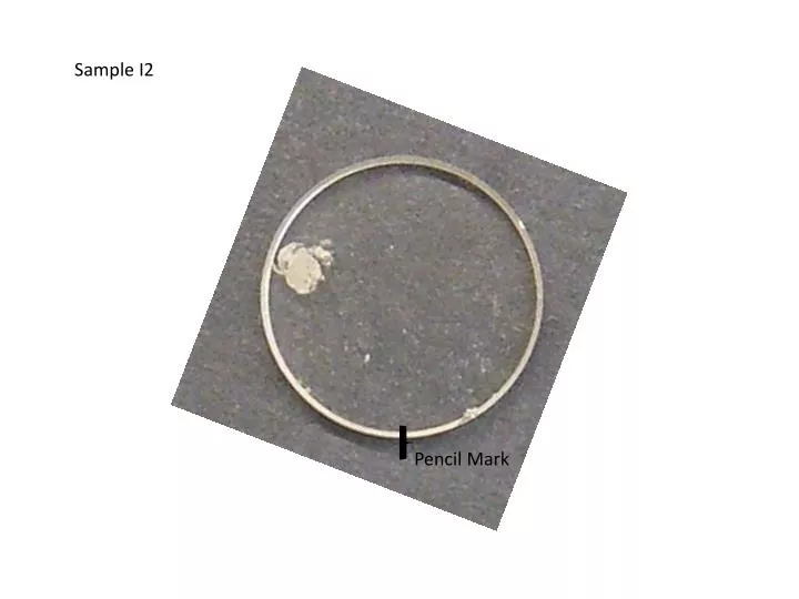
Sample I2. Pencil Mark. On this figure are marked various regions of interest, which are given letters to distinguish them. It is planned to start with region A. The general plan for Barretts sample is to: First image a 340 x 340 um “ B arrett’s” area, shown here are area A

E N D
Sample I2 Pencil Mark
On this figure are marked various regions of interest, which are given letters to distinguish them. It is planned to start with region A.
The general plan for Barretts sample is to: • First image a 340 x 340 um “Barrett’s” area, shown here are area A • Next is to zoom down (to 42x42 um?) within this area to look are the Barrett’s. This should/might manifest itself as small spheres in our topographic images. Shown on slide 5 are several sizes of boxes representing the size of 42x42 um images and 85x85 um. The exact location of these boxes should be determined by examination of our SNOM images (the exception is the box around the stroma). • After we are fairly sure we have good images of Barrett’s, we might obtain an image of the stroma. An area thought to be stroma is shown in slide 5. • You will note that there are other area of Barretts shown in slide 2, which we migth explore.
Sample I2, Area a -- 340 mm I2-2x 2 mm
I2a-8x Sample I2, Area a 340 mm 42 mm Stroma 85 mm Smaller areas inside area A are included to show possible scan areas and sizes. 500 mm
Sample I2, Area a I2a-8x-Microscope Image 340 mm Topography (#33) 42 mm Stroma * * 85 mm Smaller areas inside area A are included to show possible scan areas and sizes. 500 mm
Sample I2, Area a I2a-8x-Microscope Image 340 mm 8.05 mm raw image w/ processing 42 mm Stroma * * 85 mm 32_Sample_i2_1a_8_05_340m_32_ADC2 Smaller areas inside area A are included to show possible scan areas and sizes. 500 mm
Sample I2, Area a I2a-8x-Microscope Image 340 mm 7.30 mm raw image w/ processing 42 mm Stroma * * 85 mm 33_Sample_i2_1a_7_30_340m_33_ADC2 Smaller areas inside area A are included to show possible scan areas and sizes. 500 mm
Sample I2, Area a I2a-8x-Microscope Image 340 mm Topography (#33) 42 mm Stroma * * 85 mm Smaller areas inside area A are included to show possible scan areas and sizes. 500 mm
Calib2.0x – line spacing is 0.5 mm (17.84 cm / 2000 um) * 340 um = 3.03 cm * 85 um = 0.76 cm * 42 um = 0.37 cm
Calib8.0x – line spacing is 0.5 mm (17.36 cm / 500 um) * 340 um = 11.08 cm * 85 um = 2.95 cm * 42 um = 1.48 cm