Experience of using the Stan software for Bayesian inference in HIV epidemiology

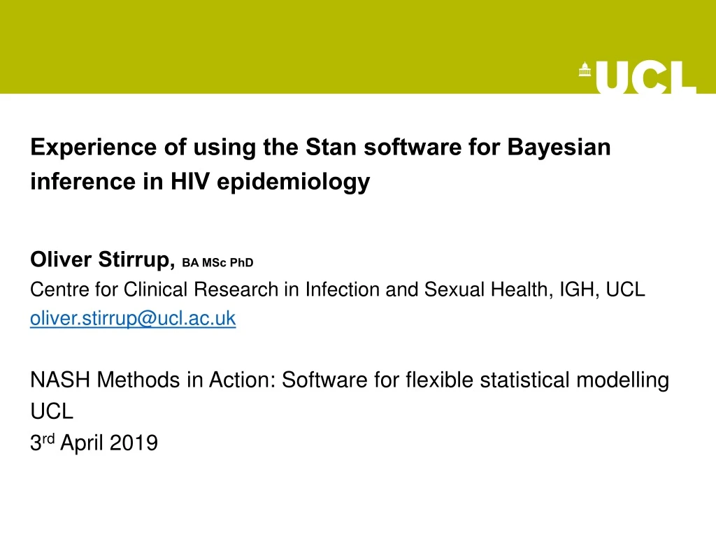
1. Experience of using the Stan software for Bayesian inference in HIV epidemiology Oliver Stirrup, BA MSc PhD Centre for Clinical Research in Infection and Sexual Health, IGH, UCLoliver.stirrup@ucl.ac.uk NASH Methods in Action: Software for flexible statistical modelling UCL 3rd April 2019

2. Structure of session • Background information on the Stan software • Practical introduction to installing and using Stan through R • Two examples of my own analyses

3. Background information • Stan is a software platform for Bayesian inference. • Named in honour of Stanislaw Ulam(credited as inventor of Monte Carlo methods). • First launched 2012. • Under active development*, but key functions are stable. • Further information and documentation: https://mc-stan.org/ • All free and open-source! • *There is now a large multinational team of developers, I am in no way involved

4. Background information • Usage still on upward trajectory: • Carpenter B et al.. Stan: A probabilistic programming language. Journal of statistical software. Jan. 2017 [accepted 2015]. Updated 22 Feb 2019

5. Background information • Use limited so far in applied health research. Top classifications for 341 citations on Web of Science: Adding up sub-categories of applied medical research I get a total of 37 papers (with two of them mine). Updated 22 Feb 2019

6. Technical details • Stan is based on C++, and user-defined models require compilation into an executable file in order to run. • Using R, Stan itself can be downloaded through CRAN in the normal way as the ‘rstan’ package. • If using a Windows computer, the Rtools software also needs to be installed separately to provide a C++ toolchain (this should be simple but requires admin rights/ IT approval…). • Installed and fairly easy to use on the UCL Research IT Services Linux cluster computing systems (Legion/Myriad).

7. Basic principles • Stan is primarily designed for sampling from the full posterior distribution in Bayesian analyses. • Models are defined by the user through template files, giving huge flexibility in model structure. • Sampling from the posterior is based on Hamiltonian Monte Carlo (HMC) (‘borrowed’ from particle physics). • HMC can provide huge improvements in computational efficiency over conventional Metropolis-Hastings and Gibbs sampling (e.g. WinBUGS/JAGS), but mathematical foundations are more difficult to follow.

8. Basic principles • As to be expected, Stan is based on Bayes’ theorem: • To create a model the Stan user just needs to define their parameters and data structure, and the (unnormalised) log joint probability density, i.e.:

9. Basic principles • In Stan (and Bayesian analysis in general), there is no distinction between conventional model parameters and unobserved ‘random effect’ terms that are included in joint distribution: • Stan requires the log joint probability density to be a smoothly differentiable function of the model parameters (and random effects).

10. Basic principles • Stan cannot sample from the posterior distribution of discrete-valued parameters. • But models that use discrete parameters or random effects (e.g. mixture model of two normals) in their construction can be analysed through marginalisation. • The Stan User Manual provides examples on how to achieve this.

11. Basic principles • Performance of Stan can depend strongly on shape of the joint posterior of all parameters. • Global correlations in the posteriors of parameters (as in multivariate normal) do not cause problems, but complex curvature can lead to poor efficiency and errors. • Problems can often be fixed by adjustment of parameterisation or priors, but this takes a little practice • For example in a mixed effects type model it is best to declare random effect terms as following a standard normal distribution and to then multiply by a scale parameter (non-centred parameterisation).

12. Basic Stan example • Very simple illustrative model: • Obtain posterior distribution of mean and variance for eight observations: • 9.7, 9.1, 9.8, 10.0, 10.1, 9.3, 9.8, 10.6 • Using priors:

13. Basic Stan example • Models defined through template files: • data { • … • } • parameters { • … • } • transformed parameters { • … • } • model{ • … • }

14. Basic Stan example • Models defined through template files: • data { • int<lower=0> J; // number of observations • real y[J]; // vector of J observations • } • parameters { • real mu; // mean parameter • real<lower=0>sigma_2; // variance parameter • } • transformed parameters { • real sigma =sqrt(sigma_2); // SD parameter • } • model { • y ~ normal(mu, sigma); // log-PDF of observations | parameters • sigma_2 ~ exponential(1); // Prior log-PDF for variance parameter • mu ~ normal(10,1); // Prior log-PDF for mean parameter • }

15. Basic Stan example • Models defined through template files: • data { • int<lower=0> J; // number of observations • real y[J]; // vector of J observations • } • parameters { • real mu; // mean parameter • real<lower=0>sigma_2; // variance parameter • } • transformed parameters { • real sigma =sqrt(sigma_2); // SD parameter • } • model { • target += normal_lpdf(y | mu, sigma); // log-PDF of observations | paras • target += exponential_lpdf(sigma_2 | 1);// Prior log-PDF for variance para • target += normal_lpdf(mu | 10, 1); // Prior log-PDF for mean para • }

16. Basic Stan example • The ‘rstan’ package can be used to feed data into a Stan model and save the resulting output: • library("rstan") • example_data<-list(J =8, • y =c(9.7, 9.1, 9.8, 10.0, 10.1, 9.3, 9.8, 10.6) • ) • fit1 <-stan(file='example1.stan', data=example_data) • The ‘stan’ R-function compiles and runs the model, with defaults: 4 chains of 2000 iterations each (half of these ‘burn-in’).

17. Basic Stan example • The ‘rstan’ package also includes functions for analysing the samples from the posterior distribution obtained: • ‘n_eff’ is effective sample size, based on observed autocorrelation of posterior samples. • ‘Rhat’ is potential scale reduction statistic, based on ratio of within-chain to overall variance of samples, should be near 1.0 when chains have all converged to same stationary distribution

18. Basic Stan example • The posterior samples can be plotted for analysis or diagnostic checks: • stan_trace(fit1, pars=c("mu","sigma_2"), inc_warmup=TRUE)

19. Basic Stan example • The posterior samples can be plotted for analysis or diagnostic check: • stan_hist(fit1, pars=c("mu","sigma_2"))

20. Basic Stan example • The posterior samples can be plotted for analysis or diagnostic check: • stan_plot(fit1, pars=c("mu","sigma_2"), ci_level=0.95)

21. Applied example 1 • Methodological project I published last year:Stirrup OT, Dunn DT. Estimation of delay to diagnosis and incidence in HIV using indirect evidence of infection dates. BMC Med Res Methodol 2018; 18: 65. doi: 10.1186/s12874-018-0522-x. • Minimisation of Dx delay critical to good outcomes in HIV patients and to limit onward infection. • Unless a patient has a history of regular testing, infection date can be very uncertain.

22. Applied example 1 • CD4+ cell counts are a type of white blood cell that are depleted over time in HIV infection.

23. Applied example 1 • Other biomarkers may also provide useful information regarding timing of infection: • -Viral load • -Viral genetic diversity Viral load Viral genetic diversity Kouyos R et al.. Ambiguous nucleotide calls from population-based sequencing of HIV-1 are a marker for viral diversity and the age of infection. Clin Infect Dis.2011; 52: 532-9.

24. Applied example 1 • Problem of estimating Dx delays is tied to problem of estimating incidence of new infections. • For a limited period of time observing new diagnoses, the distribution of observed Dx delays is affected by any change in incidence. • Therefore, we want to model HIV incidence and Dx delay jointly.

25. Applied example 1 • Discrete time and stage models currently used to calculate underlying incidence. Sweeting MJ et al. Bayesian back-calculation using a multi-state model with application to HIV. Statistics in Medicine 2005; 24: 3991-4007.

26. Applied example 1 • Methods: First fit joint model for biomarkers in seroconverters, relative to true time of infection. • True time of HIV infection is treated as a random variable in each patient, with assumed uniform prior over possible dates in seroconverters. • Summarise approximate posterior of biomarker model parameters using a multivariate normal. • Use this to fit joint model for biomarker data, Dx delay and incidence in a population of ‘seroprevalent’ patients (without testing history)

27. Applied example 1 • Joint model for incidence and Dx delay: • - Infections occur according to a Poisson process for which the rate of new events is an intensity function of time h(x) • - Dx delays follow a time-to-event distribution • Incidence-Dx-delay model developed based on work of Medley et al. (1987,1988), who analysed time-to-AIDS from HIV infection at transfusion. Medley GF, Anderson RM, Cox DR, Billard L. Incubation period of AIDS in patients infected via blood transfusion. Nature. 1987; 328: 719–21. Medley GF, Billard L, Cox DR, Anderson RM. The distribution of the incubation period for the acquired immunodeficiency syndrome (AIDS). Proc R SocLond B Biol Sci. 1988; 233: 367–77.

28. Applied example 1 • The marginal log-PDF includes expression of the form: • Unless incidence (h(x)) is constant, the need for an analytic solution to A limits our choice of survival distribution. • An exponential survival distribution can be combined with pragmatic choices for incidence function. Calendar time at infection Delay to Dx Survival density Incidence function End and beginning of observation period for Dx

29. Applied example 1 • We can construct a full PDF for incidence and Dx delay parameters (λ) and Dx delays in individual patients (τ), the biomarker data in each patient (y) and the prior distribution for biomarker model parameters (p(θ)) from the analysis of seroconverters: • ]

30. Applied example 1 • Model fitted to cohort data for ‘men who have sex with men’ in London diagnosed HIV+ 2009-2013 (n=3521 patients): Estimated mean time to Dx (95% CrI): • ‘White’ ethnicity: 1.57 (1.41–1.75) yearsn=2577 • ‘Other’ ethnicity: 2.68 (2.04–3.45) yearsn=705 • ‘Black’ ethnicity: 2.91 (1.92–4.76) yearsn=239 Four chains of 1250 iterations and warm-up of 500 iterations, giving 3000 samples from the posterior. Run in parallel on UCL Legion cluster with ‘wall-clock’ time of 19 hours.

31. Example of individual patient predictions • Patient diagnosed in 2013 and a viral sequence sampled at time of Dxshowed ambiguous nucleotide calls at 0.66% of positions. CD4 cell counts of 300 and 295 cells/µL and VL of 30 000 and 58 000 copies/mL were recorded at time of Dxand 40 days later, respectively.

32. Example of individual patient predictions • Patient diagnosed in 2009 and a viral sequence 12 days after Dxshowed no ambiguous nucleotide calls. The first three CD4 cell counts obtained were 615, 875 and 800 cells/µL at 12, 140 and 260 days after diagnosis, and the first three VL measurements were 320,000, 630 and 2500 copies/mL at 10, 140 and 430 days after diagnosis.

33. Applied example 2 • Current applied project:Does use of emtricitabine (FTC) or lamivudine (3TC) following detection of the M184V HIV resistance mutation reduce the incidence of further drug resistance • Context: -HIV now treated with combination drug therapy • -HIV can develop resistance to specific drugs • -The M184V mutation confers high-level resistance to FTC/3TC • -But, the M184V mutation itself may reduce ability of HIV to develop further resistance mutations

34. Applied example 2 • Analysis conducted using the UK Collaborative HIV Cohort (UK CHIC) and UK HIV Drug Resistance Database • Inclusion criteria: change to drug regimen (/treatment initiation) within 1 year of first detection of M184V mutation. • Patients followed-up until further change to drug regimen. • Objective: to evaluate whether use of 3TC/FTC use is associated with incidence of new HIV drug resistance mutations.

35. Applied example 2 • Dataset: 2164 patients with 957 (44%) on 3TC/FTC, median follow-up 1.2 years (IQR 0.4-2.9 years). • Data collected over ≈20 year period with 684 distinct drug regimens. • Numerous other potentially confounding factors: CD4+ cell count, viral load, number of other resistance mutations, mode of infection, age, clinical centre (n≈40)…

36. Applied example 2 • Poisson model most obvious for count data, but I condition on drug regimen to simplify the analysis. • Stratified Poisson regression leads to a multinomial PDF for events within each strata. • Use of a random effect term by clinical centre would probably be tractable in marginal ML analysis, but I do not think implemented in any standard software. • Selection or shrinkage for large number of predictive variables? • Standard Poisson assumes independence of events: include patient-level frailty term?

37. Applied example 2 • My model in Stan: • - Conditional Poisson stratified by drug regimen • - Regression coefficients follow Laplace distribution with data-driven scale parameter (diffuse hyperprior) • - Normally distributed random effects for clinical centre on log-hazard scale (diffuse hyperprior for variance) • - Normally distributed frailty term on log-hazard scale (diffuse hyperprior for variance) • Eight chains of 800 iterations and warm-up of 300 iterations, giving 4000 samples from the posterior. Run in parallel on UCL Legion cluster with ‘wall-clock’ time of 4 minutes.

38. Applied example 2 • Key result: based on our modelling assumptions, use of 3TC/FTC is probably associated with a reduction in the rate of new drug resistance mutations. • IRR: 0.49, 95% CrI 0.18-1.00 • Probability(IRR<1)=0.975

39. Stan pros and cons • Extremely flexible • Full Bayesian inference • State of the art MC sampling • Good documentation • Strong helpful online community • Active and open development • Free and open-source • Cross platform • Integration with R/Stata/Python • Requires C++ toolchain to use • Requires users to write out own models • Debugging and optimising models takes some practice • Not easy to acquire intuition of theoretical basis of MC routines • Compilation time (2-3 min) slows down simple models

40. Full Bayes pros, cons and other thoughts • Easy to incorporate different information sources • Arguably more robust and intuitive than some classical approaches • Extra work choosing priors • Can be harder to convince Reviewers and Editors • Tends to require more thought • Less likely to produce strong results with realistic priors: good for science, bad for publication? • Flexibility removes computational excuses for simple models

41. Links and references (practical) Stan homepage: https://mc-stan.org/ rstanquick-start guide: https://github.com/stan-dev/rstan/wiki/RStan-Getting-Started Stan reference manual: https://mc-stan.org/docs/2_18/reference-manual/ -includes exact details of n_eff and Rhat estimators (under ‘Posterior Analysis’) General introduction: Carpenter B, Gelman A, Hoffman MD, Lee D, Goodrich B, Betancourt M, et al.. Stan: a probabilistic programming language. J Stat Softw2017; 76: 32.

42. Links and references (theoretical) Betancourt M. A conceptual introduction to Hamiltonian Monte Carlo. arXiv preprint arXiv:1701.02434. 2017 Jan 10. Scalable Bayesian Inference with Hamiltonian Monte Carlo - Michael Betancourt: https://icerm.brown.edu/video_archive/?play=1107 (or any other Michael Betancourt intro to Hamiltonian Monte Carlo videos). Another introduction video describing intuition for Hamiltonian Monte Carlo (Ben Lambert of Imperial, also has some intro to Bayes and Stan videos): https://www.youtube.com/watch?v=a-wydhEuAm0.