Download
1 / 60
600 likes | 683 Views
Material Functions. Part 3 Introduction to the Rheology of Complex Fluids. To find constitutive equations, experiments are performed on materials using standard flows. stress responses → materials & type of flow time strain strain rate (or other kinematic parameters)

E N D
Material Functions Part 3 Introduction to the Rheology of Complex Fluids
To find constitutive equations, experiments are performed on materials using standard flows. stress responses → materials & type of flow time strain strain rate (or other kinematic parameters) chemical nature of the material Numerous standard flows may be constructed from the two sets of flows, by varying the functions σ(t) and ε(t) (and b) functions of the kinematic parameters that characterize the rheological behavior are material functions
Material Functions Definitions of material functions consist of three parts: • Choice of flow type • Details of the σ(t) and ε(t) (and b) that appear in the definition of the flows. • Material function definitions – based on the measured stress quantities
Material Functions To predict them: • Use the kinematics and const. eq. to predict the stress components • Calculate the material functions To measure them: • Impose the kinematics on material in a flow cell • Measure the stress components To choose a constitutive equation to describe a material, we need both to measure the material function and to predict it.
Steady Shear Kinematics for steady shear constant • Produced in a rheometer by: • Forcing the fluid through a capillary at a constant rate and the steady pressure required to maintain the flow is measured. • Using cone-and-plate and parallel-plate geometry, rotate at constant angular velocity while measuring the torque generated by the fluid.
Steady-State Shear For S.S., the stress tensor is constant in time, and the three stress quantities are measured. The three material functions that are defined are: Either + or -, depending on the flow direction and the choice of coordinate system. Viscosity First normal-stress coefficient Second normal stress coefficient Zero-shear viscosity
Steady-State Shear Either + or -, depending on the flow direction and the choice of coordinate system. shear rate strain stress
Unsteady Shear Made in the same geometries as steady shear. Measured pressures and torques are functions of time. Many types of time-dependent shear flows: • Shear-stress growth • Shear-stress relaxation/decay • Shear creep • Step shear strain • Small-amplitude oscillatory shear
Shear-Stress Growth • Before steady-state is reached, there is a start-up portion of the experiment in which the stress grows from its zero at-rest value to the steady-state value. • This start-up experiment is one time-dependent shear flow experiment no flow initially Kinematics for shear-stress growth may be positive or negative
Shear-Stress Growth The three material functions that are defined are: Viscosity First normal-stress growth coefficient Second normal-stress growth coefficient
Shear-Stress Growth At steady-state these material functions become steady-state functions: Viscosity First normal-stress growth coefficient Second normal-stress growth coefficient
Shear-Stress Growth shear rate strain stress
Shear-Stress Decay • Relaxation properties of non-Newtonian fluids may be obtained by observing how the steady-state stresses in shear flow relax when the flow is stopped. may be positive or negative Kinematics for shear-stress decay no flow initially
Shear-Stress Decay The three material functions are analogous to stress growth and are defined as: Viscosity First normal-stress decay coefficient Second normal-stress decay coefficient
Shear-Stress Decay shear rate strain stress
Shear-Stress Decay • Newtonian fluids relax instantaneously when the flows stops. • For many Non-Newtonian fluids relaxation takes a finite amount of time. • The time that characterizes a material’s stress relaxation after deformation is called the relaxation time, λ. • A dimensionless number that is used to characterize the importance of λ is the Deborah number De material relaxation time flow time scale Deborah number can help predict the response of a system to a particular deformation.
Deborah Number – An unusual interpretation The prophetess Deborah said: “The mountains flowed before the Lord” (Judges 5:5) The interpretation of Prof. Markus Reiner: Deborah knew two things: 1. Mountains flow as everything flows. 2. But they flowed before the Lord, not before man Reiner’s interpretation: “Man in his short lifetime cannot see them flowing, while the time of observation of God is infinite.” Thus, even some solids “flow” if they are observed long enough. Reiner, M. “The Deborah Number,” Physics Today, pp 62, January, 1964.
Shear Creep An alternative way of producing steady shear flow is to drive the flow at constant stress. Constant driving pressure in a capillary flow, or by driving the fixtures with a constant-torque motor. The unsteady response to shear flow when a constant stress is imposed is necessarily different from the response when a constant strain rate is imposed. In the constant-stress experiment, the time-dependent deformation of the sample is measured during the transient flow. The unsteady shear experiment where the stress is held constant is called creep.
Shear Creep • The material function will prescribe the stress: Prescribed stress function for creep In creep deformation of a sample is measured, that is how the sample changes shape over some time interval as a result of the imposition of the stress. To do that the concept of strain must be defined.
Shear Creep • To measure deformation we use the shear strain. • Strain is a measure of the change of the shape of a fluid particle, that is, how much stretching or contracting a fluid experiences. • Shear strain is denoted by γ21(tref, t) • Refers to the strain at time t with respect to the shape of the fluid particle at some other time (i.e. tref) • may be abbreviated as γ21(t), where tref = 0 • For short time intervals: where u1 is the displacement function in the 1-direction Shear Strain (small deformations)
Shear Creep Then the displacement function is: u1 is just the 1-direction component
Shear Creep Physical Interpretation: is the slope of the side deformed particle Thus, strain is related to the change in shape of a fluid particle in the vicinity of points P1 and P2.
Shear Creep For steady shear flow over short time intervals, the particle position vector is: where r is the initial particle position and the velocity is For steady simple shear flow over a short time interval from 0 to t then, we calculate the displacement function and strain: Strain in steady-shear over short interval
Shear Creep The deformation in the creep experiment occurs over a long time interval, and the previous equation is for small deformations is not sufficient for calculating strain in this flow. However, we can break a large strain into a sequence of N smaller strains: where tp = pΔt and Δt = t/N. The steady shear-flow displacement function is given for short time intervals by: Therefore, for each small-strain interval, independent of time
Shear Creep The total strain over the entire interval from 0 to t is given by: Same results as for short time intervals and it is valid in steady-shear flows. For creep, an unsteady flow, the relationship between γ21(0,t) and the measured shear rate is a bit more complicated since the shear rate varies with time. The displacement function is the same, however is replaced by the measured time-dependent shear rate function Now we will consider the general case of strain between two times t1 and t2.
Shear Creep Break the interval into N pieces of duration Δt: The strain for each interval is: With varies with time. Thus, for unsteady shear flow, a large strain between times t1 and t2 is given by:
Shear Creep In the limit Δt goes to zero This expression for strain is valid in unsteady shear flows such as creep. Shear strain in the creep experiment may be obtained by measuring the instantaneous shear rate as a function of time and integrating it over the time interval.
Shear Creep In creep because the stress is prescribed rather than measured, the material functions relate the measured sample deformation (strain) to the prescribed stress. The creep compliance is: The creep compliance curve has many features, and several other material functions related to it can be defined.
Shear Creep Steady-state compliance is defined as the difference between the compliance function at a particular time at steady-state and t/η, the steady-flow contribution to the compliance function at that time: Creep recovery – when the driving stress is removed, elastic and viscoelastic materials will spring back in the opposite direction to the initial flow direction, and the amount of strain that is recovered is called the steady-state recoverable shear strain or recoil strain. Sample is constrained such that no recovery takes place in the 2-direction.
Shear Creep Recoverable Creep Compliance Recoil Function Recoverable Shear Ultimate recoil function
Shear Creep For small stresses (i.e. linear viscoelastic limit) the strain at all times is just the sum of the strain that is recoverable and the strain that is not recoverable (due to steady viscous flow at infinite time) Nonrecoverable shear strain due to steady shear flow the shear rate attained at s.s. in creep experiment • Advantages to creep flow: • more rapid approach to steady-state • Creep-recovery gives important insight into elastic memory effects • Sometimes materials are sensitive to applied stress levels rather than shear-rate levels • It is straightforward to determine critical stresses
Step Shear Strain One of the interesting properties of polymers and other viscoelastic materials is that they have partial memory (stresses that do not relax immediately but rather decay over time) . The decay is a kind of memory time or relaxation time for the fluid. To investigate relaxation time, one of the most commonly employed experiments is the step-strain experiment in shear flow. Kinematics of step shear strain The limit expresses that the shearing should occur as rapidly as possible. The condition __ relates to the magnitude of the shear strain imposed.
Step Shear Strain As previously discussed: Taking the time derivative and applying Leibnitz rule: For step-strain experiment: It is called the step-strain experiment: this flow involves a fixed strain applied rapidly to a test sample at time t=0.
Step Shear Strain The prescribed shear-rate function in terms of the strain is: Where the function multiplying the strain is an asymmetric impulse or delta function Thus we can write:
Step Shear Strain The strain can be expressed: Heaviside step function
Step Shear Strain The response of a non-Newtonian fluid to the imposition of a step strain is a rapid increase in shear and normal stresses followed by a relaxation of these stresses. The material functions are based on the idea of modulus rather than viscosity. Modulus is the ratio of stress to strain and is a concept that is quite useful for elastic materials. Relaxation modulus First normal-stress step shear relaxation modulus Second normal-stress step shear relaxation modulus
Step Shear Strain The second normal stress … modulus is seldom measured since it is small and requires specialized equipment. For small strain, the moduli are found to be independent of strain, this limit is called the linear viscoelastic regime. In the linear viscoelastic regime G(t,strain) is written as G(t), and often high strain data are reported relative to G(t) through the use of a material function called the damping function: only reported when it is independent of time.
Small-Amplitude Oscillatory Shear One of the most common material functions set. The flow is again shear flow, and the time-dependent shear-rate function used for this flow is periodic (a cosine function). Kinematics for SAOS frequency (rad/s) constant amplitude of the shear rate function Usually done (but not limited to) in parallel plate or cone-and-plate.
Small-Amplitude Oscillatory Shear From the strain, the wall motion required to produce SAOS can be calculated. Small shear strains can be written as If b(t) is the time-dependent displacement of the upper plate (for example) and h the gap between the plates And strain can be calculated from the strain rate: strain amplitude
Small-Amplitude Oscillatory Shear Thus the motion of the wall is: Moving the wall of a shear cell in a sinusoidal manner does not guarantee that the shear-flow velocity profile will be produced, but one can show that a linear velocity profile will be produced for sufficiently low frequencies or high viscosities.
Small-Amplitude Oscillatory Shear When a sample is strained at low strain amplitudes, the shear stress that is produced will be a sine wave of the same frequency as the input strain wave. The shear stress usually will not be in phase with the input strain. It can be expressed as: Expanding using trigonometric identities: there is a portion of the stress wave that is in phase with the imposed strain (sen) and a portion of the stress wave that is in phase with the strain rate (cos)
Small-Amplitude Oscillatory Shear - Significance • Newtonian fluids: stress is proportional to shear rate. • For elastic materials: • shear stress is proportional to the imposed strain, that is to the deformation • similar to mechanical springs (which generate stress that is proportional to the change in length) Hooke’s law (shear only) The stress response generated in SAOS has both a Newtonian-like and an elastic part. Thus, SAOS is ideal for probing viscoelastic materials (i.e. materials that show both viscous and elastic properties)
Small-Amplitude Oscillatory Shear SAOS material functions portion of the stress wave that is in phase with the strain wave divided by the amplitude of the strain wave storage modulus portion of the stress wave that is out of phase with the strain wave divided by the amplitude of the strain wave loss modulus
Small-Amplitude Oscillatory Shear – The Limits For a Newtonian fluid, the response is completely in phase with the strain rate: For an elastic solid that follows Hooke’s law (a Hookean solid) , the shear stress response is completely in phase with the strain.
Small-Amplitude Oscillatory Shear Several other material functions related to G’ and G” are also used by the rheological community, although they contain no information not already present in the two dynamic moduli already defined. Table 5.1
Material Functions for Elongational Flow Based on the velocity field: Only the stress differences can be measured. Stress measurements are very challenging to make in elongational geometries. In many experiments flow birefringence is used. Flow birefringence is an optical property that is proportional to stress. Measurements of strain are sometimes made by videotaping a marker particle in the flow and analyzing the images using computer software.
Steady Elongation Steady-state elongational flow is produced by choosing the following kinematics: For these flows, constant stress differences are measured. The material functions defined are two elongational viscosities based on the measured normal stress-differences. For both uniaxial and biaxial extension, the elongational viscosity base on t22-t11 is zero for all fluids. uniaxial elongational viscosity biaxial elongational viscosity
Steady Elongation Steady-state elongational flow is difficult to achieve because of the rapid Rate of particle deformation that is required. Very few reliable data are available for this important flow. The strain in elongational flow is defined as: Integrating: Hencky strain