Download
1 / 1
10 likes | 110 Views
DYNAMICAL AND STATISTICAL CHARACTERISTICS OF ATMOSPHERIC DUST DEVILS. Michael Kurgansky A.M. Obukhov Institute of Atmospheric Physics, Moscow, RUSSIA E-mail: kurgansk@ifaran.ru. European Geosciences Union General Assembly 2011

E N D
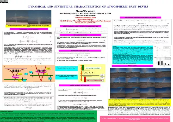
DYNAMICAL AND STATISTICAL CHARACTERISTICS OF ATMOSPHERIC DUST DEVILS Michael Kurgansky A.M. Obukhov Institute of Atmospheric Physics, Moscow, RUSSIA E-mail: kurgansk@ifaran.ru European Geosciences Union General Assembly 2011 AS1.5/NP.10/OS2.6 "Recent Developments in Geophysical Fluid Dynamics" Vienna, Austria, April 04, 2011 Size-frequency distribution of atmospheric dust devils Kurgansky (2006) proposed that terrestrial dust devil observations are best fit byan exponential function of the form (6) (a) (b) Two characteristic morphological forms of dust devils: (a) rope-type vortices and (b) vase-type vortices where P is the probability that the dust devil size exceeds a given diameter D, and the decay parameter D1 is approximately twice the Obukhov length scale L0; i.e., D12L0. For example, the size–frequency distribution of dust devils observed in the Tucson Basin and Avra Valley by Sinclair (1966) is best fit by D1 = 8.3 m, and the dust devil density observed in the Mojave Desert by Carroll and Ryan (1970) can be reproduced by D1 = 1.7 m (Kurgansky, 2006). General equation of balance of helicity in a Boussinesq fluid Two asymptotic vortex solutions Here, F is any force, e.g. due to friction; S denotes the helicity flux vector. For a steady axisymmetricinviscid flow this general balance equation (Kurgansky, 2008) is equivalent to Eq. (2). However, Lorenz (2009) argues that such an exponential distribution does not provide a good match to MER observations of Martian dust devils (Greeley et al., 2006). Instead, Lorenz demonstrates that a simple power law distribution, the cumulative form of which can be expressed as In polar cylindrical (r,,z) coordinates, two integral formulas follow from the non-linear thermal wind equation for a steady axisymmetric inviscid flow of a Boussinesq fluid, above a surface-adjacent turbulent viscous layer: Downward helicity flux (7) (1) For Helical Rankine Vortex #2 the downward helicity flux S across the top of the viscous boundary layer, at z, reads where N is the number of dust devils per sq. km per day exceeding diameter D, and k250 km2daym, better fits the MER observations (see Fig. 1 of Lorenz (2009)). (5) Pathare et al. (2010) assessed these competing exponential and power law hypotheses of dust devil size–frequency distributions with new field observations from two sites in the southwestern United States: at diameters less than 12 m the observed dust devil size–frequency distributions are better fit by an exponential function than by a power law formulation. (2) With good accuracy Eq. (5) is applicable to Helical Rankine Vortex #1; a minor discrepancy results from a very weak artificial upward flux of the helicity across the singular level z=h . Here, b is the buoyancy; v=(u,v,w) and =(r,,z) are the velocity and the vorticity vectors; z1 and z2 are two arbitrary altitudinal levels. Helical parameter is similar but not identical to the ‘relative helicity’ defined by the cosine of the angle between the vectors of velocity and vorticity. The downward helicity flux S strictly vanishes for ||, where || corresponds to the helical ‘Beltrami flow’. FIGURE 3. (A) Cumulative number of dust devils N exceeding a given diameter D. Filled circles correspond to the survey of 528 dust devils in Eldorado Valley: error bars represent standard sqrt(N) error. For the A = 0.55 km2 survey area, the cumulative form (short-dashed line, R2 = 0.838) of the power law distribution (Eq. (7)) does not fit the observations so well as the cumulative form (long-dashed line, R2 = 0.999) of the exponential function for D1 = 4.6 m (derived by multiplying P in Eq. (6) by k in Eq. (7), in order to enable direct comparison with the power law formulation. (B) Histogram showing differential dust devil size distribution, expressed as a percentage of the total number of dust devils observed/predicted in each diameter bin. From left to right (within each diameter bin) bars correspond to: Eldorado survey of 528 dust devils; exponential function (Eq. (6)); and power law (via Eq. (7)). The value of the decay parameter that produces the best fit to the observed Eldorado differential distribution is D1 = 4.6 m (R2 = 0.98). The exponential function (Eq. (6)) provides an excellent match to the Eldorado field observations across all four diameter bins. FROM: Pathare et al. , 2010; Figure 1 and legend to it. Helical Rankine Vortex #1: the similarity assumptions are used when the relative distribution of velocity components is the same across the vortex at all altitudes. The rotational velocity v at each horizontal level has a profile which is characteristic for a Rankine vortex with irrotational flow periphery. The vertical velocity w in the vortex core corresponds to an updraft flow. At each horizontal level w is uniform inside the vortex core; in the peripheral flow w. The radius of the vortex core rmz is a monotonic increasing function of altitude z. A non-linear differential equation (Kurgansky, 2005; cf. a magnetostatic problem for sunspots inSchlüter and Temesváry, 1958) Total helicity of the vortex flow Helical Rankine Vortex #2 possesses a well-defined finite total helicity value which is equal to the doubled product of the toroidal Ktvmrmand the poloidal Kpvmz0 Kelvin’s velocity circulation (cf. Moffatt, 1969). follows from Eq. (1) and describes the vortex constitution, given the angular momentum and the vertical volumetric flux Q, and provided bz were prescribed. The morphologically simplest vortex solution reads (Kurgansky, 2005) For Helical Rankine Vortex #1, the total helicity H is given by a diverging integral. or ‘Demon spawn’ (a) (b) FIGURE 1. Schematic of a dust devil vortex: Helical Rankine Vortex #1 (a) and #2 (b) FIGURE 2. Sketch of the helicity budget in Helical Rankine Vortex #2 (not in scale!) The singular level zh is associated with the top of atmospheric convective boundary layer; the earth surface is at z. The vortex solution is valid beginning with a critical height zh and should be matched to the viscous solution for z. If applied to the level z, it yields Energy budget of the vortex flow Kinetic energy balance equation in a Boussinesq fluid (the mean fluid density ; is the non-hydrostatic pressure) (3) The helical parameter wvmis the reciprocal of the ‘swirl ratio’ (see Davies-Jones, 1973); Eq. (1) for the maximum wind speed vm is reminiscent of the ‘thermodynamical speed limit’ (e.g., Rennó et al. 1998) but contains important dependence on -parameter. shows that the kinetic energy generation rate G for Helical Rankine Vortex #2 equals to Helical Rankine Vortex #2: a swirling warm buoyant plume with irrotational poloidal flow component (u,w) is ejected from a ‘virtual’ source of mass, which is located at zz0, i.e. beneath the earth surface. The azimuthal component of vorticity has -singularity at the plume edge When ambient and vortex conditions are perfect, one or more secondary vortices may be produced adjacent to the primary column. In this case a large (30 m), poorly structured dust-laden column is accompanied with a tightly-organized, small (1m) ‘tube’ column at the leading edge of the advancing system. The smaller column rotated in the counter direction to the main vortex and it wrapped around the larger column. By placing the chase truck between them the delicately balanced air-flow was disrupted and the smaller vortex was dissipated [see Metzger S, Kurgansky V, Montecinos A, Villagran V, Verdejo H, ”Chasing dust devils in Chile’s Atacama Desert”, Lunar & Planetary Science Conference, Houston, USA, March 2010]. In a steady vortex flow, G equals to the kinetic energy viscous dissipation rate D and, as a function of the helical parameter , reaches its maximum value for () and identically vanishes elsewhere. The rotational velocity v at each horizontal level has the same profile as in Helical Rankine Vortex #1; the vortex core is congruent to the plume. The vortex solution has a physical meaning at z (z0).For this slender vortex and in full conformity with Eq. (3), Eq. (1) gives at z: For characteristic parameter values vmms, wvm ms, rmm, kgm it yields that GDkW . For the Carnot thermodynamic efficiency of the vortex as a heat engine, this power is explained by the total turbulent sensible heat flux of density 400 Wm (cf. Kurgansky et al., 2011) across a circular ground area of radius Rm, which is concentric to the dust devil vortex. REFERENCES: Carroll JJ, Ryan JA (1970) J Geophys Res 75: 5179-5184; Davies-Jones RP (1973) J Atmos Sci 30: 1427-1430; Greeley R and 13 colleagues (2006) J Geophys Res 111: E12S09(1-16); Kurgansky MV (2005) Dyn Atmos Oceans 40: 151-162; Kurgansky MV (2006) Geophys Res Lett 33: L19S06(1-4); Kurgansky MV (2008) Izvestiya Atmos Ocean Physics 44: 64-71; ; Kurgansky MV, Montecinos A, Villagran V, Metzger SM (2011) Boundary-Layer Meteorol 138: 285–298; Lorenz RD (2009) Icarus 203: 683–684; Moffatt HK (1969) J Fluid Mech 35: 117-129; Pathare AV, Balme MR, Metzger SM, Spiga A, Towner MC, Rennó NO, Saca F (2010) Icarus 209: 851–853; Rennó NO, Burkett ML, Larkin MP (1998) J Atmos Sci 55: 3244-3252; Rotunno R (1980) J Fluid Mech 97: 623-640; Sinclair PC (1966) PhD dissertation The Univ of Arizona 292 pp; Schlüter A, Temesváry S (1958) IAU Symposium No.6: Electromagnetic Phenomena in Cosmical Physics, Cambridge Univ Press pp. 263-274. (4) • CONCLUDING REMARKS: • A novel vortex solution is proposed to describe the constitution of atmospheric dust devils above the regions affected by the ground surface. This vortex model nicely fits rope-type dust devils, in distinction to more turbulent vase-type dust devils. The kinetic energy and helicity budget of the flow is analyzed and reveals realistic features of the proposed vortex model. • The vortex core structure depends primarily on the characteristics of the boundary layer feeding it (cf. Rotunno, 1980) so that the core radius scales according to the boundary layer thickness, which is an order of the Obukhov scale length L0 (cf. Kurgansky et al. 2011). It is indicative on the fact that the size-frequency distribution of dust devils should contain the parametric dependence on L0; exponential distribution (6) has this property. Scale-independent power law distributions, as well as (7), are arguably applicable to large (and usually observed remotely) dust devils, for which the pure geometric factors accompanying their monitoring and detection may also matter. The work was supported by the Russian Foundation for Basic Research, project No. 10-05-00100, and by FONDECYT (Chile) under grant 1085095 .