Download
1 / 31
310 likes | 507 Views
Chapter 4 Evaluating Classification and Predictive Performance. Introduction. In supervised learning, we are interested in predicting the class (classification) or continuous value (prediction) of an outcome variable. In the previous chapter, we worked through a simple example.

E N D
Chapter 4 Evaluating Classification and Predictive Performance
Introduction • In supervised learning, we are interested in predicting the class (classification) or continuous value (prediction) of an outcome variable. In the previous chapter, we worked through a simple example. • Let's now examine the question of how to judge the usefulness of a classifier or predictor and how to compare different ones.
Judging Classification Performance • The need for performance measures arises from the wide choice of classifiers and predictive methods. • Not only do we have several different methods, but even within a single method there are usually many options that can lead to completely different results. • A simple example is the choice of predictors used within a particular predictive algorithm. • Before we study these various algorithms in detail and face decisions on how to set these options, we need to know how we will measure success.
Accuracy Measures • A natural criterion for judging the performance of a classifier is the probability for making a misclassification error. • Misclassification • The observation belongs to one class, but the model classifies it as a member of a different class. • A classifier that makes no errors would be perfect • Do not expect to be able to construct such classifiers in the real world • Due to “noise” • Not having all the information needed to precisely classify cases.
Accuracy Measures • Is there a maximal probability of misclassification we should require of a classifier? • We hope to do better than the naive rule • “classify everything as belonging to the most prevalent class." • This rule does not incorporate any predictor information and relies only on the percent of items in each class. • If the classes are well separated by the predictor information, then even a small dataset will suffice in finding a good classifier • If the classes are not separated at all by the predictors, even a very large dataset will not help.
Shows a small dataset (n=24 observations) where two predictors (income and lot size) are used for separating owners of lawn mowers from non-owners.
Shows a much larger dataset (n=5000 observations) where the two predictors (income and average credit card spending) do not separate the two classes well (loan acceptors/non-acceptors).
Accuracy Measures • Most accuracy measures are derived from the classification matrix (also called the confusion matrix.) • This matrix summarizes the correct and incorrect classifications that a classifier produced for a certain dataset. • Rows and columns of the confusion matrix correspond to the true and predicted classes respectively. • Example follows
The above shows an example of a classification (confusion) matrix for a two-class (0/1) problem resulting from applying a certain classifier to 3000 observations. The two diagonal cells (upper left, lower right) give the number of correct classifications, where the predicted class coincides with the actual class of the observation. The off-diagonal cells give counts of misclassification. The top right cell gives the number of class 1 members that were misclassified as 0's (in this example, there were 85 such misclassifications). Similarly, the lower left cell gives the number of class 0 members that were misclassified as 1's (25 such observations). The classification matrix gives estimates of the true classification and misclassification rates. Of course, these are estimates and they can be incorrect, but if we have a large enough dataset and neither class is very rare, our estimates will be reliable.
Accuracy Measures • To obtain an honest estimate of classification error, we use the classification matrix that is computed from the validation data. • We first partition the data into training and validation sets by random selection of cases. • We then construct a classifier using the training data, • Apply it to the validation data, • Yields predicted classifications for the observations in the validation set. • We then summarize these classifications in a classification matrix. • Different accuracy measures can be derived from the classification matrix. • Example follows
Consider a two-class case with classes C0 and C1 (e.g., buyer/non-buyer). The schematic classification matrix above uses the notation ni,j to denote the number of cases that are class Ci members, and were classified as Cj members. If i <> j then these are counts of misclassifications. The total number of observations is n = n0,0 + n0,1 + n1,0 + n1,1.
Accuracy Measures • A main accuracy measure is the estimated misclassification rate, • Also called the overall error rate . • It is given by • Err = (n0,1 + n1,0)/n • where n is the total number of cases in the validation dataset • In the example above we get Err = (25+85)/3000 = 3 .67% . • If n is reasonably large, our estimate of the misclassification rate is probably reasonably accurate • We can compute a confidence interval using the standard formula for estimating a population proportion from a random sample . • The example that follows gives an idea of how the accuracy of the estimate varies with n .
In the table above the column headings are values of the misclassification rate and the rows give the desired accuracy in estimating the misclassification rate as measured by the half-width of the confidence interval at the 99% confidence level For example, if we think that the true misclassification rate is likely to be around 0.05 and we want to be 99% confident that Err is within + or - 0:01 of the true misclassification rate, we need to have a validation dataset with 3,152 cases We can measure accuracy by looking at the correct classifications instead of the misclassifications . The overall accuracy of a classifier is estimated by Accuracy = 1 - Err = (n0,0 + n1,1)/n In the example above we have (201+2689)/3000 = 96 .33%
Cutoff For Classification • Many data mining algorithms classify a case in a two-step manner: • First they estimate its probability of belonging to class 1, • Then they compare this probability to a threshold called a cut off value. • If the probability is above the cutoff, the case is classified as belonging to class 1, and otherwise to class 0. • If more than two classes, a popular rule is to assign the case to the class to which it has the highest probability of belonging. • The default cutoff value in two-class classifiers is 0.5. • If the probability of a record being a class 1 member is greater than 0.5, that record is classified as a 1. • Any record with an estimated probability of less than 0.5 would be classified as a 0. • It is possible, however, to use a cutoff value that is either higher or lower than 0.5. • A cutoff greater than 0.5 will end up classifying fewer records as 1's • A cutoff less than 0.5 will end up classifying more records as 1. • The misclassification rate will rise in either case. • Following example illustrates this
The above table contains the actual class for 24 records, sorted by the probability that the record is a 1 (as estimated by a data mining algorithm). If we adopt the standard 0.5 as the cutoff, our misclassification rate is 3/24 If we adopt instead a cutoff of 0.25 we classify more records as 1's and the misclassification rate goes up (comprising more 0's misclassified as 1's) to 5/24 If we adopt a cutoff of 0.75, we classify fewer records as 1's and the misclassification rate goes up (comprising more 1's misclassified as 0's) to 6/24. All this can be seen in the classification tables that follow
Performance in Unequal Importance of Classes • Suppose that the two classes are asymmetric • More important to predict membership correctly in class 0 than in class 1 • An example is predicting the financial status (bankrupt/solvent) of firms • It may be more important to correctly predict a firm that is going bankrupt than to correctly predict a firm that is going to stay solvent • The classifier is essentially used as a system for detecting or signaling bankruptcy • The overall accuracy is not a good measure for evaluating the classifier • There are several possible accuracy measures • The next slide lists them
Measures of AccuracyAsymmetric Classes • If the important class is C0 - Popular accuracy measures are: • Sensitivity of a classifier is its ability to correctly detect the important class members. This is measured by n0,0=(n0,0 + n0,1), the % of C0 members correctly classified • Specificity of a classifier is its ability to correctly rule out C1 members. This is measured by n1,1=(n1,0 + n1,1), the % of C1 members correctly classified. • The false positive rate is n1,0=(n0,0 + n1,0). Notice that this is a ratio within the column of C0 predictions, i.e. it uses only records that were classified as C0 . • The false negative rate is n0,1=(n0,1 + n1,1). Notice that this is a ratio within the column of C1 predictions, i.e. it uses only records that were classified as C1
Measures of AccuracyAsymmetric Classes • It is sometimes useful to plot these measures v.s. the cutoff value (using one-way tables in Excel), in order to find a cutoff value that balances these measures . • A graphical method that is very useful for evaluating the ability of a classifier to "catch" observations of a class of interest is the lift chart . • We describe this in further detail next
Lift Charts • Useful when classifying rare events • Tax cheats, debt defaulters, or responders to a mailing. • Our classification model is to sift through the records • Sort them according to which ones are most likely to be tax cheats, responders to the mailing, etc. • We can then make more informed decisions. • We can decide how many tax returns to examine, looking for tax cheats. • The model will give us an estimate of the extent to which we will encounter more and more non-cheaters as we proceed through the sorted data. • Or we can use the sorted data to decide to which potential customers a limited-budget mailing should be targeted. • We are describing the case when our goal is to obtain a rank ordering among the records rather than actual probabilities of class membership.
Lift Charts • When the classifier gives a probability of belonging to each class and not just a binary classification to C1 or C0, we use the lift curve • also called a gains curve or gains chart. • The lift curve is a popular technique in direct marketing. • Consider a data mining model that attempts to identify the likely responders to a mailing by assigning each case a “probability of responding" score. • The lift curve helps us determine how effectively we can “skim the cream" by selecting a relatively small number of cases and getting a relatively large portion of the responders. • The input required to construct a lift curve is a validation dataset that has been “scored" by appending to each case the estimated probability that it will belong to a given class
We've shown that different choices of a cutoff value lead to different confusion matrices Instead of looking at a large number of classification matrices, it is much more convenient to look at the cumulative lift curve (sometimes called a gains chart) which summarizes all the information in these multiple classification matrices into a graph.
The graph is constructed with the cumulative number of cases (in descending order of probability) on the x-axis and the cumulative number of true positives on the y-axis True positives are those observations from the important class (here class 1) that are classified correctly. The table of cumulative values of the class 1 classifications and the corresponding lift chart. The line joining the points (0,0) to (24,12) is a reference line. For any given number of cases (the x-axis value), it represents the expected number of positives we would predict if we did not have a model but simply selected cases at random. It provides a benchmark against which we can see performance of the model.
Lift Charts • If we had to choose 10 cases as class 1 (the important class) members and used our model to pick the ones most likely to be 1's, the lift curve tells us that we would be right about 9 of them. • If we simply select 10 cases at random we expect to be right for 10 X 12/24 = 5 cases. The model gives us a “lift" in predicting class 1 of 9/5 = 1.8. • The lift will vary with the number of cases we choose to act on. • A good classifier will give us a high lift when we act on only a few cases (i.e. use the prediction for the ones at the top). • As we include more cases the lift will decrease. • The lift curve for the best possible classifier - a classifier that makes no errors - would overlap the existing curve at the start, continue with a slope of 1 until it reached 12 successes (all the successes), then continue horizontally to the right.
The same information can be portrayed as a “decile" chart, shown above, which is widely used in direct marketing predictive modeling. • The bars show the factor by which our model outperforms a random assignment of 0's and 1's. • Reading the first bar on the left, we see that taking the 10% of the records that are ranked by the model as “the most probable 1's" yields twice as many 1's as would a random selection of 10% of the records. • XLMiner automatically creates lift (and decile) charts from probabilities predicted by classifiers for both training and validation data. • Of course, the lift curve based on the validation data is a better estimator of performance for new cases
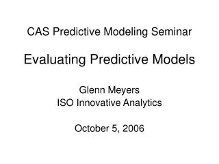
ROC Curve (Receiver Operating Characteristic) It is worth mentioning that a curve that captures the same information as the lift curve in a slightly different manner is also popular in data mining applications. It uses the same variable on the y-axis as the lift curve (but expressed as a percentage of the maximum) and on the x-axis it shows the true negatives (the number of unimportant class members correctly classified, also expressed as a percentage of the maximum) for differing cutoff levels. The ROC curve for our 24 cases example above is shown in Figure 4.9.