Download
1 / 46
460 likes | 610 Views
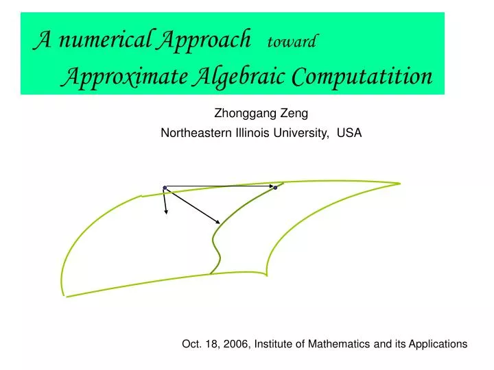
A numerical Approach toward Approximate Algebraic Computatition. Zhonggang Zeng Northeastern Illinois University, USA. Oct. 18, 2006, Institute of Mathematics and its Applications. What would happen when we try numerical computation on algebraic problems?.

E N D
A numerical Approachtoward Approximate Algebraic Computatition Zhonggang Zeng Northeastern Illinois University, USA Oct. 18, 2006, Institute of Mathematicsand its Applications
What would happen when we try numerical computation on algebraic problems? A numerical analyst got a surprise 50 years ago on a deceptively simple problem. 1
Start of project: 1948 Completed: 1950 Add time: 1.8 microseconds Input/output: cards Memory size: 352 32-digit words Memory type: delay lines Technology: 800 vacuum tubes Floor space: 12 square feet Project leader: J. H. Wilkinson Britain’s Pilot Ace James H. Wilkinson (1919-1986) 2
The Wilkinson polynomial p(x) = (x-1)(x-2)...(x-20) = x20 - 210 x19 + 20615 x18 + ... Wilkinson wrote in 1984: Speaking for myself I regard it as the most traumatic experience in my career as a numerical analyst. 3
approximation A factorable polynomial irreducible Factoring a multivariate polynomial: 6
Translation: There are two 1-dimensional solution set: Solving polynomial systems: Example: A distorted cyclic four system: 7
approximation Isolated solutions 1-dimensional solution set Distorted Cyclic Four system in floating point form: 8
tiny perturbation in data (< 0.00000001) huge error In solution ( >105 ) 9
What could happen in approximate algebraic computation? • “traumatic” error • dramatic deformation of solution structure • complete loss of solutions • miserable failure of classical algorithms • Polynomial division • Euclidean Algorithm • Gaussian elimination • determinants • … … 10
Either or So, why bother with approximation in algebra? • You may have no choice (e.g. Abel’s Impossibility Theorem) All subsequent computations become approximate 11
blurred image blurred image true image Application: Image restoration (Pillai & Liang) So, why bother with approximation solutions? • You may have no choice • Approximate solutions are better!
blurred image blurred image restored image Application: Image restoration (Pillai & Liang) true image Approximate solution is better than exact solution! 13
Approximate solutions by Bertini (Courtesy of Bates, Hauenstein, Sommese, Wampler) Perturbed Cyclic 4 Exact solutions by Maple: 16 isolated (codim 4) solutions
Perturbed Cyclic 4 Exact solutions by Maple: 16 isolated (codim 4) solutions Or, by an experimental approximate elimination combined with approximate GCD Approximate solutions are better than exact ones , arguably 15
Special case: Example: JCF computation Maple takes 2 hours On a similar 8x8 matrix, Maple and Mathematica run out of memory So, why bother with approximation solutions? • You may have no choice • Approximate solutions are better • Approximate solutions (usually) cost less • You may have no choice • Approximate solutions are better • Approximate solutions (usually) cost less 16
Pioneer works in numerical algebraic computation (incomplete list) • Homotopy method for solving polynomial systems • (Li, Sommese, Wampler, Verschelde, …) • Numerical Algebraic Geometry • (Sommese, Wampler, Verschelde, …) • Numerical Polynomial Algerba • (Stetter) 17
exact computation approximate solution using 8-digits precision forward error backward error axact solution - - - = 2 4 2 ( x 1 ) ( 10 ) 0 What is an “approximate solution”? To solve with 8 digits precision: backward error: 0.00000001 -- method is good forward error: 0.0001 -- problem is bad 18
From problem From numerical method The condition number [Forward error] < [Condition number] [Backward error] A large condition number <=> The problem is sensitive or, ill-conditioned An infinite condition number <=> The problem is ill-posed 19
Wilkinson’s Turing Award contribution: Backward error analysis • A numerical algorithm solves a “nearby” problem • A “good” algorithm may still get a “bad” answer, if the problem is ill-conditioned (bad) 20
Ill-posed problems are common in applications • image restoration - deconvolution • IVP for stiction damped oscillator - inverse heat conduction • some optimal control problems - electromagnetic inverse scatering • air-sea heat fluxes estimation - the Cauchy prob. for Laplace eq. • … … • A well-posed problem: (Hadamard, 1923) • the solution satisfies • existence • uniqueness • continuity w.r.t data An ill-posed problem is infinitely sensitive to perturbation tiny perturbation huge error 21
- Multiple roots - Polynomial GCD - Factorization of multivariate polynomials - The Jordan Canonical Form - Multiplicity structure/zeros of polynomial systems - Matrix rank Ill-posed problems are common in algebraic computing 22
Ill-posed problems are infinitely sensitive to data perturbation A numerical algorithm seeks the exact solution of a nearby problem If the answer is highly sensitive to perturbations, you have probably asked the wrong question. Maxims about numerical mathematics, computers, science and life, L. N. Trefethen. SIAM News Does that mean: (Most) algebraic problems are wrong problems? Conclusion: Numerical computation is incompatible with ill-posed problems. Solution: Formulate the right problem. 23
Solution P P Data P Challenge in solving ill-posed problems: Can we recover the lost solution when the problem is inexact? P:Data Solution 24
William Kahan: This is a misconception Are ill-posed problems really sensitive to perturbations? Kahan’s discovery in 1972: Ill-posed problems are sensitive to arbitrary perturbation, but insensitive to structure preserving perturbation. 25
W. Kahan’s observation (1972) • Problems with certain solution structure form a “pejorative manifold” Plot of pejorative manifolds of degree 3 polynomials with multiple roots Why are ill-posed problems infinitely sensitive? • The solution structure is lost when the problem leaves the manifold due to an arbitrary perturbation • The problem may not be sensitive at all if the problem stays on the manifold, unless it is near another pejorative manifold 26
Geometry of ill-posed algebraic problems Similar manifold stratification exists for problems like factorization, JCF, multiple roots … 27
Manifolds of 4x4 matrices defined by Jordan structures (Edelman, Elmroth and Kagstrom 1997) e.g. {2,1} {1} is the structure of 2 eigenvalues in 3 Jordan blocks of sizes 2, 1 and 1 28
? B A ? perturbation Problem A Problem B Illustration of pejorative manifolds The “nearest” manifold may not be the answer The right manifold is of highest codimension within a certain distance 29
Finding approximate solution is (likely) a well-posed problem Approximate solution is a generalization of exact solution. A “three-strikes” principle for formulating an “approximate solution” to an ill-posed problem: • Backward nearness: The approximate solution is the exact solution of a nearby problem • Maximum codimension: The approximate solution is the exact solution of a problem on the nearby pejorative manifold of the highest codimension. • Minimum distance: The approximate solution is the exact solution of the nearest problem on the nearby pejorative manifold of the highest codimension. 30
Formulation of the approximate rank /kernel: Backward nearness:app-rank of A is the exact rank of certain matrix B within q. The approximate rank of A within q : Maximum codimension:That matrix B is on the pejorative manifold P possessing the highest co-dimension and intersecting the q-neighborhoodof A. The approximate kernel of A within q : with Minimum distance:That B is the nearest matrix on the pejorative manifold P. • An exact rank is the app-rank within sufficiently small q. • App-rank is continuous (or well-posed) 31
= 4 nullity = 2 = 4 nullityq = 2 After reformulating the rank: Rank Rankq Ill-posedness is removed successfully. kernel App-rank/kernel can be computed by SVD and other rank-revealing algorithms (e.g. Li-Zeng, SIMAX, 2005) basis + eE = 6 nullity = 0 + eE = 4 nullityq = 2 32
The AGCD within e : Formulation of the approximate GCD • Finding AGCD is well-posed if qk(f,g) is sufficiently small • EGCD is an special case of AGCD for sufficiently small e(Z. Zeng, Approximate GCD of inexact polynomials, part I&II) 33
Similar formulation strikes out ill-posedness in problems such as • Approximate rank/kernel(Li,Zeng 2005, Lee, Li, Zeng 2006) • Approximate multiple roots/factorization(Zeng 2005) • Approximate GCD(Zeng-Dayton 2004, Gao-Kaltofen-May-Yang-Zhi 2004) • Approximate Jordan Canonical Form(Zeng-Li 2006) • Approximate irreducible factorization(Sommesse-Wampler-Verschelde 2003, Gao et al 2003, 2004, in progress) • Approximate dual basis and multiplicity structure(Dayton-Zeng 05, Bates-Peterson-Sommese ’06) • Approximate elimination ideal(in progress) 34
after formulating the approximate solution to problem P within e Stage I: Find the pejorative manifold P of the highest dimension s.t. P P S Stage II: Find/solve problem Q such that Q The two-staged algorithm Exact solution of Q is the approximate solution of P within e which approximates the solution of S where P is perturbed from 35
Stage II: solve the (overdetermined) quadratic system for a least squares solution (u,v,w) by Gauss-Newton iteration Case study: Univariate approximate GCD: Stage I: Find the pejorative manifold (key theorem: The Jacobian of F(u,v,w) is injective.) 36
Max-codimension k := k-1 k := k-1 Is AGCD of degree k possible? no no probably Refine with G-N Iteration Successful? yes Min-distance nearness Output GCD Start: k = n Univariate AGCD algorithm 37
Stage II: solve the (overdetermined) quadratic system for a least squares solution (u,v,w) by Gauss-Newton iteration (key theorem: The Jacobian of F(u,v,w) is injective.) Case study: Multivariate approximate GCD: Stage I: Find the max-codimension pejorative manifold by applying univariate AGCD algorithm on each variable xj 38
Stage II: solve the (overdetermined) polynomial system F(z1 ,…,zk )=f (in the form of coefficient vectors) for a least squares solution (z1 ,…,zk) by Gauss-Newton iteration (key theorem: The Jacobian is injective.) Case study: univariate factorization: Stage I: Find the max-codimension pejorative manifold by applying univariate AGCD algorithm on (f, f’ ) 39
A ~ J l 1 l 1 l J = Segre characteristic = [3,1] B l A codim = -1 + 3 + 3(1) = 5 l l s13 s23 s14 s24 s34 Wyre characteristic = [2,1,1] lI+S= l l 3 1 2 1 1 Ferrer’s diagram Case study: Finding the nearest matrix with a Jordan structure P Equations determining the manifold 40
A ~ J B A For B not on the manifold, we can still solve for a least squares solution : When is minimized, so is of is injective. The crucial requirement: The Jacobian (Zeng & Li, 2006) Case study: Finding the nearest matrix with a Jordan structure Equations determining the manifold P 41
Project to tangent plane u1 = G(z0)+J(z0)(z1- z0) ~ tangent plane P0 : u = G(z0)+J(z0)(z- z0) Least squares solution u*=G(z*) new iterate u1=G(z1) initial iterate u0=G(z0) Solving G(z) = a a Pejorative manifold u = G( z ) Solve G( z ) = a for nonlinear least squares solutionz=z* Solve G(z0)+J(z0)(z - z0 ) = a for linear least squares solutionz =z1 G(z0)+J(z0)(z - z0 ) = a J(z0)(z - z0 ) = - [G(z0) - a ] z1 = z0 - [J(z0)+][G(z0) - a] 42
condition number (sensitivity measure) Stage I: Find the nearby max-codim manifold Stage II: Find/solve the nearest problem on the manifold via solving an overdetermined system G(z)=a for a least squares solutionz* s.t . ||G(z*)-a||=minz ||G(z)-a|| by the Gauss-Newton iteration Key requirement: Jacobian J(z*) of G(z) at z* is injective (i.e. the pseudo-inverse exists) 43
univariate/multivariate GCDmatrix rank/kernel dual basis for a polynomial ideal univariate factorization irreducible factorizationelimination ideal … … (to be continued in the workshop next week) Summary: • An (ill-posed) algebraic problem can be formulated using the three-strikes principle (backward nearness, maximum-codimension, and minimum distance) to remove the ill-posedness • The re-formulated problem can be solved by numerical computation in two stages (finding the manifold, solving least squares) • The combined numerical approach leads to Matlab/Maple toolbox ApaTools for approximate polynomial algebra. The toolbox consists of 44