Linkages Between Environmental Monitoring and Modeling

1. Linkages Between Environmental Monitoring and Modeling Mark Cohen NOAA Air Resources Laboratory Silver Spring, Maryland, USA Presentation at NADP 2003: Long Term Monitoring: Supporting Science and Informing Policy October 20-22, 2003 Washington Hilton, Washington DC

2. Inextricable Linkage BetweenModeling and Monitoring Modeling needed to help interpret measurements and estimate source-receptor relationships Monitoring needed to develop models and to evaluate their accuracy

3. Two Main Approaches in Linking Modeling and Monitoring • Challenges in Exploiting Synergisms Between Modeling and Monitoring

4. Two Main Approachesin LinkingModeling & Monitoring • Receptor-Oriented Methods • (e.g., Back Trajectory Analysis) 2. Comprehensive Fate and Transport Models based on Emissions Inventories

5. Receptor-Oriented Methods • Back Trajectory Analysis • Start with measurements at a given location • Use meteorology to estimate back trajectories of air parcels constituting each measurement • Can develop estimates of relative importance of different source regions in influencing concentrations at the site • Enhancements include Cluster Analysis; • and Potential Source Contribution Function (PSCF) Analysis

6. Receptor-Oriented Methods • Advantages of Back-Trajectory Analyses • Emissions inventory not needed • Relatively simple calculations – little computational resources required • Don’t need information about fate processes

7. Receptor-Oriented Methods • Difficulties with Back-Trajectory Analyses • Need a lot of measurements • Measurements must be short duration • (e.g., a few hours or at most a day) • Can’t start back trajectory at the ground • (where the measurement was made) • must “guess” where to start the back-trajectory (500, 1000 meters?) • ...answers will be influenced by this decision • Not sure where on the back trajectories • the important sources really are • Very difficult to account for fate processes (deposition, chemical transformation)

8. Receptor-Oriented Methods • Chemical Mass Balance Methods • Start with emissions profiles of different source categories • Determine what proportion of contributions from each source category would be required to match the existing measurements • Yields estimates of the impact of these different source categories at the measurement site

9. Receptor-Oriented Methods • Difficulties with Chemical Mass Balance Methods • Emissions profiles for different source categories not always known • Need measurements of many different pollutants to carry out analysis • Don’t get information about the spatial extent of the significant sources • Fate processes not accounted for • (e.g., chemical transformation)

10. Receptor-Oriented Methods • Summary • Receptor-oriented measurements can provide limited source-receptor information • With no emissions inventory, • its all you can do…

11. Two Main Approachesin LinkingModeling & Monitoring • Receptor-Oriented Methods • (e.g., Back Trajectory Analysis) 2. Comprehensive Fate and Transport Models based on Emissions Inventories

12. Comprehensive Fate and Transport Models Based on Emissions Inventories Geographic distribution of total mercury emissions to the atmosphere from U.S. and Canadian anthropogenic sources (1995/1996). (Speciation?) • Methodology • Start with emissions inventory

13. Comprehensive Fate and Transport Models Based on Emissions Inventories • Methodology • Start with emissions inventory • Incorporate atmospheric behavior of pollutant(s) into 3-D fate & transport model: • Phase-partitioning • Chemical transformation • Wet and dry deposition

14. Atmospheric Fate Processes for Hg Elemental Mercury: Hg(0) Reactive Gaseous Mercury: RGM Particulate Mercury: Hg(p) Halogen-mediated oxidation on the surface of ice crystals cloud cloud droplet Hg(II) reduced to Hg(0) by SO2 and sunlight Hg(0) oxidized to RGM by O3, H202, Cl2, OH, HCl Hg(p) Adsorption/ desorption of Hg(II) to /from soot “DRY” (low RH) ATMOSPHERE Hg(0) oxidized to dissolved RGM by O3, HOCl, OCl- Primary Anthropogenic Emissions Re-emission of natural AND previously deposited anthropogenic mercury Dry and Wet Deposition

15. Atmospheric Chemical Reaction Scheme for Mercury

16. Comprehensive Fate and Transport Models Based on Emissions Inventories • Methodology • Start with emissions inventory • Incorporate atmospheric behavior of pollutant(s) into 3-D fate & transport model: • Phase-partitioning • Chemical transformation • Wet and dry deposition • Provide model with meteorology • Simulate the fate and transport of emissions, keeping track of the impact of different sources on receptors of interest • Evaluate model by comparison against monitoring data... • (improve model if necessary and possible)

17. Atmospheric Fate Processes for Hg Elemental Mercury: Hg(0) Reactive Gaseous Mercury: RGM Particulate Mercury: Hg(p) Halogen-mediated oxidation on the surface of ice crystals cloud cloud droplet Hg(II) reduced to Hg(0) by SO2 and sunlight Hg(0) oxidized to RGM by O3, H202, Cl2, OH, HCl Hg(p) Adsorption/ desorption of Hg(II) to /from soot “DRY” (low RH) ATMOSPHERE Hg(0) oxidized to dissolved RGM by O3, HOCl, OCl- Primary Anthropogenic Emissions Re-emission of natural AND previously deposited anthropogenic mercury Dry and Wet Deposition To what extent is Hg(p) soluble?

18. Soluble Hg(p) Insoluble Hg(p)

19. Soluble Hg(p) Insoluble Hg(p)

20. Comprehensive Fate and Transport Models Based on Emissions Inventories • Methodology • Start with emissions inventory • Incorporate atmospheric behavior of pollutant(s) into 3-D fate & transport model: • Phase-partitioning • Chemical transformation • Wet and dry deposition • Provide model with meteorology • Simulate the fate and transport of emissions, keeping track of the impact of different sources on receptors of interest • Evaluate model by comparison against monitoring data; improve model if necessary and possible • If evaluation shows results are reasonable, report source-receptor information

21. Comprehensive Fate and Transport Models Based on Emissions Inventories • Advantages • Can potentially develop detailed source-receptor information

22. Figure A. Geographic distribution of contributions to atmospheric deposition of mercury to Lake Superior (g/km2-yr).

23. Percent of total estimated emissions and model-estimated deposition of mercury to the Great Lakes contributed from different distance ranges away from each lake.

24. Per-capita mercury contributions to the Great Lakes from U.S. and Canadian sources (ng Hg deposited per km2 of lake surface per person per year); “fuels” = fuel combustion; “incin” = waste incineration; “metals” = metallurgical processes; “manuf” includes “other” source types (e.g., lamp breakage) in addition to manufacturing processes (e.g., chloralkali production).

25. Comprehensive Fate and Transport Models Based on Emissions Inventories • Advantages • Can potentially develop detailed source-receptor information • Can analyze different emissions or climate scenarios • Can fill in the spatial and temporal gaps between measurements • Can estimate quantities not easily measured (e.g., dry deposition) • A test of our knowledge – if models fail, it means we still don’t know enough emissions and/or atmospheric fate phenomena…

26. Comprehensive Fate and Transport Models Based on Emissions Inventories • Difficulties • Emissions inventories uncertain & incomplete • Even if average emissions are well known, temporal variations of emissions from any given source are largely unknown • Atmospheric behavior often not well known • … so, difficult to model • High resolution meteorological data expensive (one year of met data for the U.S. at ~24 km resolution costs ~$100-200K; ~500 GB of data)

27. Comprehensive Fate and Transport Models Based on Emissions Inventories • Difficulties (continued) • Need emissions and meteorology for same time period as monitoring • Difficult to determine causes of poor model performance • Effect of sources outside the model domain • Multimedia phenomena difficult to model • How to deal with uncertainties?

28. Effect of fate simulation variations on the geographical pattern of PCDD/F deposition contributions to Lake Superior.

29. Uncertainties in model estimates of total 1996 dioxin deposition to Lake Superior.

30. Challenges in Exploiting Synergisms BetweenModelingandMonitoring

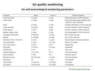
31. Challenges in Exploiting Synergisms Between Modeling and Monitoring • Data availability • Measurement data often not available (NADP/MDN are wonderful exceptions!) • Not all parameters measured to comprehensively evaluate the model: • Ambient concentrations (vs. wet deposition) • Speciation (e.g., different forms of mercury) • Vapor-particle partitioning • Size distribution of particulate pollutant • Data above ground level • Measurements in clouds

32. Challenges in Exploiting Synergisms Between Modeling and Monitoring • Emissions inventory not precisely known • Meteorology very complex (flow around buildings) • Spatial Scale of Data • Measurement data may not be appropriate for model use (e.g., urban measurements not useful to evaluate large-scale comprehensive models)

33. Challenges in Exploiting Synergisms Between Modeling and Monitoring • Spatial Scale of Data • Measurement data may not be appropriate for model use (e.g., urban measurements not useful to evaluate large-scale comprehensive models) • Corollary: If monitoring location near intense source, then unrealistically accurate characterization of that source and detailed micro-meteorology of near-field region needed

34. Sampling site? • Sampling near intense sources? • Must get the fine-scale met “perfect” • Not really a relevant test Ok, if one wants to develop hypotheses regardingwhether or not this is actually a sourceof the pollutant (and you can’t do a stack test for some reason!).

35. Challenges in Exploiting Synergisms Between Modeling and Monitoring • Spatial Scale of Data • Measurement data may not be appropriate for model use (e.g., urban measurements not useful to evaluate large-scale comprehensive models) • Corollary: If monitoring location near intense source, then unrealistically accurate characterization of that source and detailed micro-meteorology of near-field region needed • Grid-average model results difficult to compare with point measurements

36. Eulerian grid models givegrid-averaged values –…difficult to compare against measurement at a single location

37. Challenges in Exploiting Synergisms Between Modeling and Monitoring • Temporal Scale of Data • Short term measurements needed for receptor-oriented approaches • But, short-term measurements can confound comprehensive emissions-based modeling systems

39. Challenges in Exploiting Synergisms Between Modeling and Monitoring • Collaboration Issues • Timing issue: measurements made “now”; emissions inventories to support comprehensive modeling not available for many years • Competition between measurements and modeling for scarce resources • This competition affects data availability…

40. Monitoring is absolutely essential, but it cannot provide all the answers we need Models can be used to obtain additional information from monitoring data Measurements are used directly in receptor-oriented modeling approaches Measurements are essential for ground-truthing comprehensive modeling approaches Measurements can be used to improve models although a wider range of measurements would be even more helpful There are challenges in linking models and monitoring, but if all monitoring programs were like the NADP and MDN, the linkages would be greatly facilitated... Summary

42. Extra Slides

43. In the first version of the HYSPLIT-Hg model used in this intercomparison, Hg(p) was assumed to be completely converted to dissolved Hg(II) whenever a particle becomes a droplet (e.g., above approximately 80% relative humidity); and dissolved Hg(II) assumed to become Hg(p) whenever the droplet dries out • Hg(p) and Hg(II) were thus somewhat “equivalent” in the model • With this assumption, the model tended to underpredict Hg(p) and overpredict Hg(II), suggesting that the assumption of complete conversion was not valid. • However, it was encouraging to note that the model was getting approximately the right answer for the sum of the two forms of mercury (Hg(p) + Hg(II), representing the total pool of oxidized Hg in the atmosphere [see the following graphs]

45. As a result of this observation, the model was re-run with the assumption that Hg(p) was not soluble. With this assumption, the results for Hg(p) and RGM were dramatically better. [These new results are what have been shown in this presentation, except for the immediately preceding RGM+Hg(p) graphs] The affect of changing this assumption had a negligible impact on Hg(0), as might be expected, given the generally very low concentrations of Hg(II) and Hg(p) relative to Hg(0).

46. Figure 7. Model evaluation sites for wet deposition fluxes within 250 km of any Great Lake with available data for 1996.

50. Figure 8. Comparison of model-estimated wet deposition fluxes with measured values at sites in the vicinity of the Great Lakes during 1996.