Download
1 / 82
840 likes | 1.11k Views
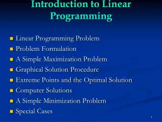
Linear Programming: Transportation Problem J. Loucks , St. Edward's University (Austin, TX, USA). Chapter 2B. Transportation Problem.

E N D
Linear Programming: Transportation ProblemJ. Loucks, St. Edward's University (Austin, TX, USA) Chapter 2B
Transportation Problem • A network model is one which can be represented by a set of nodes, a set of arcs, and functions (e.g. costs, supplies, demands, etc.) associated with the arcs and/or nodes. • Transportation problem (TP), as well as many other problems, are all examples of network problems. • Efficient solution algorithms exist to solve network problems.
Transportation Problem • TP can be formulated as linear programs and solved by general purpose linear programming codes. • For the TP, if the right-hand side of the linear programming formulations are all integers, the optimal solution will be in terms of integer values for the decision variables. • However, there are many computer packages, which contain separate computer codes for the TP which take advantage of its network structure.
Transportation Problem • The TP problem has the following characteristics: • m sources and n destinations • number of variables is m x n • number of constraints is m + n (constraints are for source capacity and destination demand) • costs appear only in objective function (objective is to minimize total cost of shipping) • coefficients of decision variables in the constraints are either 0 or 1
Transportation Problem • The transportation problem seeks to minimize the total shipping costs of transporting goods from m origins (each with a supply si) to n destinations (each with a demand dj), when the unit shipping cost from an origin, i, to a destination, j, is cij. • The network representation for a transportation problem with two sources and three destinations is given on the next slide.
Transportation Problem • Network Representation 1 d1 c11 1 s1 c12 c13 2 d2 c21 c22 2 s2 c23 3 d3 SOURCES DESTINATIONS
The Relationship of TP to LP • TP is a special case of LP • How do we formulate TP as an LP? • Let xij = quantity of product shipped from source i to destination j • Let cij = per unit shipping cost from source i to destination j • Let si be the row i total supply • Let dj be the column j total demand • The LP formulation of the TP problem is:
The Relationship of TP to LP • LP Formulation The linear programming formulation in terms of the amounts shipped from the origins to the destinations, xij, can be written as: Min SScijxij i j s.t. Sxij<si for each origin i j Sxij>dj for each destination j i xij> 0 for all i and j
Transportation Problem • LP Formulation Special Cases The following special-case modifications to the linear programming formulation can be made: • Minimum shipping guarantees from i to j: xij>Lij • Maximum route capacity from i to j: xij<Lij • Unacceptable routes: delete the variable (or put a very high cost, called the Big-M method, on a selected pair of i and j)
Transportation Problem • To solve the transportation problem by its special purpose algorithm, it is required that the sum of the supplies at the origins equal the sum of the demands at the destinations. If the total supply is greater than the total demand, a dummy destination is added with demand equal to the excess supply, and shipping costs from all origins are zero. Similarly, if total supply is less than total demand, a dummy origin is added. • When solving a transportation problem by its special purpose algorithm, unacceptable shipping routes are given a cost of +M (a large number).
Transportation Problem • The transportation problem is solved in two phases: • Phase I — Obtaining an initial feasible solution • Phase II — Moving toward optimality • In Phase I, the Minimum-Cost Procedure can be used to establish an initial basic feasible solution without doing numerous iterations of the simplex method. • In Phase II, the Stepping Stone Method, using the MODI method for evaluating the reduced costs may be used to move from the initial feasible solution to the optimal one.
Transportation Algorithm • Phase I - Minimum-Cost Method (simple and intuitive) • Step 1: Select the cell with the least cost. Assign to this cell the minimum of its remaining row supply or remaining column demand. • Step 2: Decrease the row and column availabilities by this amount and remove from consideration all other cells in the row or column with zero availability/demand. (If both are simultaneously reduced to 0, assign an allocation of 0 to any other unoccupied cell in the row or column before deleting both.) GO TO STEP 1.
Transportation Algorithm • Phase II - Stepping Stone Method • Step 1: For each unoccupied cell, calculate the reduced cost by the MODI method described below. Select the unoccupied cell with the most negative reduced cost. (For maximization problems select the unoccupied cell with the largest reduced cost.) If none, STOP. • Step 2: For this unoccupied cell generate a stepping stone path by forming a closed loop with this cell and occupied cells by drawing connecting alternating horizontal and vertical lines between them. Determine the minimum allocation where a subtraction is to be made along this path.
Transportation Algorithm • Phase II - Stepping Stone Method (continued) • Step 3: Add this allocation to all cells where additions are to be made, and subtract this allocation to all cells where subtractions are to be made along the stepping stone path. (Note: An occupied cell on the stepping stone path now becomes 0 (unoccupied). If more than one cell becomes 0, make only one unoccupied; make the others occupied with 0's.) GO TO STEP 1.
Transportation Algorithm • MODI Method (for obtaining reduced costs) Associate a number, ui, with each row and vj with each column. • Step 1: Set u1 = 0. • Step 2: Calculate the remaining ui's and vj's by solving the relationship cij = ui + vj for occupied cells. • Step 3: For unoccupied cells (i,j), the reduced cost = cij - ui - vj.
D1 D2 D3 Supply 30 20 15 S1 50 30 40 35 S2 30 Demand 25 45 10 Example 1: TP • A transportation tableau is given below. Each cell represents a shipping route (which is an arc on the network and a decision variable in the LP formulation), and the unit shipping costs are given in an upper right hand box in the cell.
Example 1: TP Building Brick Company (BBC) has orders for 80 tons of bricks at three suburban locations as follows: Northwood — 25 tons, Westwood — 45 tons, and Eastwood — 10 tons. BBC has two plants, each of which can produce 50 tons per week. How should end of week shipments be made to fill the above orders given the following delivery cost per ton: NorthwoodWestwoodEastwood Plant 1 24 30 40 Plant 2 30 40 42
Northwood Westwood Eastwood Dummy Supply 30 40 0 24 Plant 1 50 30 40 42 0 Plant 2 50 Demand 25 45 10 20 Example 1: TP • Initial Transportation Tableau Since total supply = 100 and total demand = 80, a dummy destination is created with demand of 20 and 0 unit costs.
Example 1: TP • Least Cost Starting Procedure • Iteration 1: Tie for least cost (0), arbitrarily select x14. Allocate 20. Reduce s1 by 20 to 30 and delete the Dummy column. • Iteration 2: Of the remaining cells the least cost is 24 for x11. Allocate 25. Reduce s1 by 25 to 5 and eliminate the Northwood column. • Iteration 3: Of the remaining cells the least cost is 30 for x12. Allocate 5. Reduce the Westwood column to 40 and eliminate the Plant 1 row. • Iteration 4: Since there is only one row with two cells left, make the final allocations of 40 and 10 to x22 and x23, respectively.
Example 1: TP • Iteration 1 • MODI Method 1. Set u1 = 0 2. Since u1 + vj = c1j for occupied cells in row 1, then v1 = 24, v2 = 30, v4 = 0. 3. Since ui + v2 = ci2 for occupied cells in column 2, then u2 + 30 = 40, hence u2 = 10. 4. Since u2 + vj = c2j for occupied cells in row 2, then 10 + v3 = 42, hence v3 = 32.
Example 1: TP • Iteration 1 • MODI Method (continued) Calculate the reduced costs (circled numbers on the next slide) by cij - ui + vj. Unoccupied CellReduced Cost (1,3) 40 - 0 - 32 = 8 (2,1) 30 - 24 -10 = -4 (2,4) 0 - 10 - 0 = -10
ui Northwood Westwood Eastwood Dummy 25 5 30 +8 40 20 0 24 Plant 1 0 -4 30 40 40 10 42 -10 0 Plant 2 10 vj 24 30 32 0 Example 1: TP • Iteration 1 Tableau
Example 1: TP • Iteration 1 • Stepping Stone Method The stepping stone path for cell (2,4) is (2,4), (1,4), (1,2), (2,2). The allocations in the subtraction cells are 20 and 40, respectively. The minimum is 20, and hence reallocate 20 along this path. Thus for the next tableau: x24 = 0 + 20 = 20 (0 is its current allocation) x14 = 20 - 20 = 0 (blank for the next tableau) x12 = 5 + 20 = 25 x22 = 40 - 20 = 20 The other occupied cells remain the same.
Example 1: TP • Iteration 2 • MODI Method The reduced costs are found by calculating the ui's and vj's for this tableau. 1. Set u1 = 0. 2. Since u1 + vj = cij for occupied cells in row 1, then v1 = 24, v2 = 30. 3. Since ui + v2 = ci2 for occupied cells in column 2, then u2 + 30 = 40, or u2 = 10. 4. Since u2 + vj = c2j for occupied cells in row 2, then 10 + v3 = 42 or v3 = 32; and, 10 + v4 = 0 or v4 = -10.
Example 1: TP • Iteration 2 • MODI Method (continued) Calculate the reduced costs (circled numbers on the next slide) by cij- ui + vj. Unoccupied CellReduced Cost (1,3) 40 - 0 - 32 = 8 (1,4) 0 - 0 - (-10) = 10 (2,1) 30 - 10 - 24 = -4
ui Northwood Westwood Eastwood Dummy 25 25 30 +8 40 +10 0 24 Plant 1 0 -4 30 20 40 10 42 20 0 Plant 2 10 vj 24 30 36 -6 Example 1: TP • Iteration 2 Tableau
Example 1: TP • Iteration 2 • Stepping Stone Method The most negative reduced cost is = -4 determined by x21. The stepping stone path for this cell is (2,1),(1,1),(1,2),(2,2). The allocations in the subtraction cells are 25 and 20 respectively. Thus the new solution is obtained by reallocating 20 on the stepping stone path. Thus for the next tableau: x21 = 0 + 20 = 20 (0 is its current allocation) x11 = 25 - 20 = 5 x12 = 25 + 20 = 45 x22 = 20 - 20 = 0 (blank for the next tableau) The other occupied cells remain the same.
Example 1: TP • Iteration 3 • MODI Method The reduced costs are found by calculating the ui's and vj's for this tableau. 1. Set u1 = 0 2. Since u1 + vj = c1j for occupied cells in row 1, then v1 = 24 and v2 = 30. 3. Since ui + v1 = ci1 for occupied cells in column 2, then u2 + 24 = 30 or u2 = 6. 4. Since u2 + vj = c2j for occupied cells in row 2, then 6 + v3 = 42 or v3 = 36, and 6 + v4 = 0 or v4 = -6.
Example 1: TP • Iteration 3 • MODI Method (continued) Calculate the reduced costs (circled numbers on the next slide) by cij - ui + vj. Unoccupied CellReduced Cost (1,3) 40 - 0 - 36 = 4 (1,4) 0 - 0 - (-6) = 6 (2,2) 40 - 6 - 30 = 4
ui Northwood Westwood Eastwood Dummy 5 45 30 +4 40 +6 0 24 Plant 1 0 20 30 +4 40 10 42 20 0 Plant 2 6 vj 24 30 36 -6 Example 1: TP • Iteration 3 Tableau Since all the reduced costs are non-negative, this is the optimal tableau.
Example 1: TP • Optimal Solution FromToAmountCost Plant 1 Northwood 5 120 Plant 1 Westwood 45 1,350 Plant 2 Northwood 20 600 Plant 2 Eastwood 10 420 Total Cost = $2,490
Example 2: TP Des Moines (100 units capacity) Cleveland (200 units Req.) Boston (200 units req.) Albuquerque (300 units Req.) Evansville (300 units capacity) Fort Lauderdale (300 units capacity)
Example 2: TP • What is the initial solution? • Since we want to minimize the cost, it is reasonable to “be greedy” and start at the cheapest cell ($3/unit) while shipping as much as possible. This method of getting the initial feasible solution is called the least-cost rule • Any ties are broken arbitrarily. (Des Moines to Cleveland - $3)(Evansville to Cleveland - $3)Let’s start ad cell 1-3 (Des Moines to Cleveland) • In making the flow assignments make sure not to exceed the capacities and demands on the margins!
Example 2: TP Start +100 0 100
Example 2: TP +100 +100 0 200 0 100
Example 2: TP +100 +200 +100 0 0 200 0 0 100
Example 2: TP +100 +200 +100 +300 0 0 200 0 0 0 0 100
Example 2: TP • The initial feasible solution via the least-cost rule is: • Ship 100 units from Des Moines to Cleveland • Ship 100 units from Evansville to Cleveland • Ship 200 units from Evansville to Boston • Ship 300 units from Fort Lauderdale to Albuquerque • The total cost of this solution is: • 100(3) + 100(3) + 200(4) + 300(9) = $4,100 • Is the current solution optimal? • Perhaps, but we are not sure. Hence, some more work is needed.
Example 2: TP • The cells that have a number in them are referred to as basic cells (or basic variables) • In general, all basic variables are strictly positive • When at least one basic variable is equal to zero, the corresponding solution is called degenerate • When a solution is degenerate, exercise caution in using sensitivity reports
Example 2: TP • How many basic variables (cells) should there be in the transportation tableau? • Answer: (R+C-1), where R = number of rows and C = number of columns. Here, (R+C-1) = 3+3-1 = 5 • What are they (there are 4 of them)? • Ship 100 units from Des Moines to Cleveland • Ship 100 units from Evansville to Cleveland • Ship 200 units from Evansville to Boston • Ship 300 units from Fort Lauderdale to Albuquerque
Example 2: TP • Is this solution degenerate? • Answer: Yes, because (R+C-1) = 3+3-1 = 5 > 4 • Hence, we can arbitrarily make (5-4) = 1 variable which is at level zero basic. • Let us make Des Moines to Albuquerque a basic variable at level zero • How do we determine if the current solution is optimal? • Let us price currently nonbasic variables (cells), which are all at level zero using the stepping stone algorithm
Example 2: TP 0 +100 +200 +100 +300
Example 2: TP • Evansville – Albuquerque: • 8 – 3 + 3 – 5 = 3 > 0
Example 2: TP 0 +100 +200 +100 +300
Example 2: TP • Des Moines - Boston: • 4 – 3 + 3 - 4 = 0
Example 2: TP 0 +100 +200 +100 +300
Example 2: TP • Fort Lauderdale - Boston: • 7 – 9 + 5 - 3 + 3 – 4 = -1 < 0
Example 2: TP 0 +100 +200 +100 +300