Download
1 / 50
630 likes | 945 Views
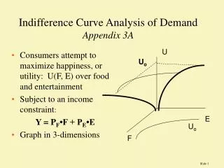
Indifference Curve Analysis. 1. A consumer is assumed to buy any two goods in combinations. 2. A consumer can rank the alternative combinations and compare their level of satisfaction, and he prefers a combination providing a higher level of satisfaction.

E N D
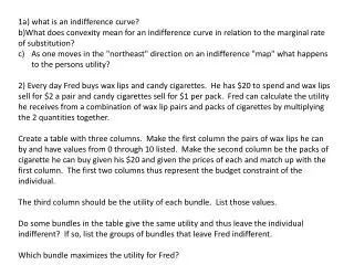
1. A consumer is assumed to buy any two goods in combinations. 2. A consumer can rank the alternative combinations and compare their level of satisfaction, and he prefers a combination providing a higher level of satisfaction. 3. Consumer is rational and his choices are transitive. 4.The consumer behaviour is assumed to be constant, throughout the analysis. 5. Indifference curve analysis assumes diminishing marginal rate of substitution. ASSUMPTION OF INDIFFERENCE CURVEANALYSIS.
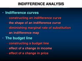
Indifference curve : A curve that shows combinations of goods among which an individual is indifferent. The slope of the indifference curve is the ratio of marginal utilities of the two goods. Indifference Curve
An indifference curve is a graph showing different bundles of goods, each measured as to quantity, between which a consumer is indifferent. That is, at each point on the curve, the consumer has no preference for one bundle over another. In other words, they are all equally preferred. One can equivalently refer to each point on the indifference curve as rendering the same level of utility(satisfaction) for the consumer. Indifference Curve
Utility is then a device to represent preferences rather than something from which preferences come. The main use of indifference curves is in the representation of potentially observable demand patterns for individual consumers over commodity bundles.
An indiffererence curve represents satisfaction of a consumer from two commodities. For all the possible points ( or combinations of the two commodities ) on an indifference curve , the total satisfaction ( or Utility) remains the same. Therefore a consumer is indifferent as to the combinations lying on an indifference curve. It is also called Iso-utility Curve. Indifference Curve.
Indifference schedule In the above schedule the consumer obtains as much Total Satisfaction from 8 Biscuits and 2 cups of tea, and same from all other combinations.
Indifference MAp • A set of indifference Curves is called Indifference map. • An indifference map is a set of indifference curves , Satisfaction level is higher the farthest indifference curve from the origin. • We cannot say how much utility the higher indifference curve represents , meaning Aggregate Utilities are rankable not measurable.
Whenever we move from one combination to another combination of the goods, we are basically substituting some units of one commodity with another. The marginal rate of substitution shows how much of one commodity is substituted for how much of another or at what rate a consumer is willing to substitute one commodity for another in his/her consumption pattern. Marginal rate of substitution
M.r.s MRS can be defined as the amount of Biscuits that is sacrificed for obtaining one Cup of Tea or as the amount of Biscuits that may be given to the consumer for the loss of one cup of Tea so that he may remain at the same level of satisfaction.
M.R.S Curve A X1/ X1B > BX2/ X2C > CX3/ X3D > DX4X4E When the consumer has just one cup of tea, he is willing to give up 4 biscuits for an additional cup of tea. Now, as the number of cups of tea increases, he is prepared to sacrifice fewer and fewer number of biscuits to get each additional cup of tea. This is due to the reason that more of one good and the less of another a consumer has, the units of the second become more important to consumer relative to the units of the first.
The indifference curves possess certain characteristics which are also called as properties. The important properties are: • 1. Downward Sloping to the right. • 2. Non-Intersecting. • 3. Convex to the Origin. Properties of indifference curve
Downward Sloping to the right orNegatively Sloped When the consumer decides to have more units of one of the two goods, he/she will have to reduce the number of the units of the other good, if he/she is to remain at the same level of satisfaction.
Upward Sloping Indifference Curve Horizontal, Vertical, Upward Sloping Indifference Curve = Absurd
Non-Intersecting No two indifference curves will cut each other. Suppose that the two indifference curves did cross , Then because point A is on the same indifference curve as point B, the two would make consumer equally happy. In addition, because point B is on the same indifference curve as point C, these two points would make the consumer equally happy. But these conclusions imply that points A & C would make the consumer equally happy even though point C has more of both goods. This contradicts our assumption that consumer prefers more of Goods than less , thus two indifference curves cannot cross.
Indifference Curves are normally convex in nature. The Implication of this convexity rule is that as we have more and more of Good X and less of Y, the marginal rate of substitution of X for Y goes on falling. Convex to origin
Concave & Straight Line Indifference Curve Concave & Straight Line Indifference Curve = Absurd or Unrealistic.
Price Line or Budget line or Budget Constraint. Higher the IC Higher is the level of satisfaction. A rational consumer will try to reach the highest possible IC in order to obtain higher level of satisfaction. In this pursuit , our consumer will be governed by the amount of the money or income he has to spend on goods and the prices of the goods in the market.
The budget line is a constraint on your choices. You can afford any point on your budget line or inside it. You cannot afford any point outside your budget line. Consumption Possibilities
A rise in the price of the good on the x-axis: Decreases the affordable quantity of that good. Causes the budget line to rotate. Increases the slope of the budget line. The budget Constraint- A change in prices
The consumer’s best affordable point is: 1. On the budget line. 2.On the highest attainable indifference curve. 3.Has a marginal rate of substitution between the two goods equal to the relative price of the two goods. Consumer’s Equillibriumor Maximising satisfaction or Optimal Choice.
Effect on consumers equilibrium of a change in consumers income, relative prices of commodities remaining same, is called Income Effect. Income effect is the effect on the quantity demanded exclusively as a result of change in money income, all prices remaining constant. As a result of change in income , his satisfaction will either increase or diminish, for he has now a larger or smaller income to spend. Income Effect
ICC for Inferior Goods Sometimes it also happens that with the rise in income, the consumer buys more of one commodity and less of another. For instance, he may buy less of wheat and more of rice. In diagram the income consumption curve bends back on itself. With the rise in income, the consumer buys more of rice and less of wheat. The price effect for rice is positive and for wheat is negative. The good which is purchased less with the increase in income is called inferior good.
Income Effect When Rice is an Inferior Good: In the figure , it is shown that with the rise in money income, the purchase of wheat has increased from M1 to M4 indicating positive income effect on the purchase of normal good wheat. The income effect on inferior good is negative. The income consumption curve ICC is starts bending towards the horizontal axis which shows that wheat is a normal good and rice is inferior good.
Price Effect on the Consumption of a Normal Good: Price Effect : PCC When there is change in the price of a good shown on the two axes of an indifference map, there takes place a change in demand in response to a change in price of a commodity, other things remaining the same, is called price effect.
Pcc FOR Normal Good AB is the initial budget line. It is assumed that the price of wheat has fallen and the price of rice and the income of the consumer remains unchanged. The price line takes a new position AC and the equilibrium point shifts from P to U.
The consumer buys now OT quantity of wheat (the amount demanded rises from OE to OT) and OZ quantity of rice. With further fall in the price of wheat, the consumer is in equilibrium at point S, where the budget line AD is tangent to a higher indifference curve IC3. He buys now OF quantity of wheat and OR quantity of rice. The rise in amount purchased of wheat (OE to OF) as a result of a fall in its price is called price effect. The price effect on the consumption of a normal good is Positive. If we join the equilibrium points PUS, we get price consumption curve (PCC) of the consumer for the commodity wheat.
PCC when Commodity is a Giffen good Giffen good is a particular type of inferior good. When there is a decrease in the quantity demanded of a good with a fall in its price, the good is called Giffen good .
The consumer is in equilibrium at point E where the budget line AB is tangent to the indifference curve IC1. The consumer purchases OX1 quantity of Giffen good X and OY1 quantity of good Y. When there is a reduction in the price of good X but no change in the price of good Y, the budget line AB/ will showing upward.The consumer is in equilibrium at point E/where the budget line AB/ is a tangent to the indifference curve IC2. In the new equilibrium position, the consumer purchases only OX2 units of Giffen good X and OY2 units of good Y. We find that the decrease in the price of Giffen good X, its quantity purchased has fallen from OX1 to OX2 and the quantity demanded of Y commodity goes up from OY1 to OY2. The price effect on the consumption of Giffen good is Negative. It is indicated by the backward bending PCC in the case of X as a Giffen good.
The decomposition of the price effect into the income and substitution effect can be done in several ways. There are two main methods: (i) The Hicksianmethod; and (ii) The Slutskymethod. Price Change: Income & Substitution Effects
THE HICKSIAN METHOD • Sir John R.Hicks (1904-1989) • Awarded the Nobel Laureate in Economics (with Kenneth J. Arrrow) in 1972 for work on general equilibrium theory and welfare economics.
THE HICKSIAN METHOD X2 Optimal bundle is Ea, on indifference curve I1. Ea I1 xa X1
THE HICKSIAN METHOD A fall in the price of X1 The budget line pivots out from P X2 P* Ea I1 xa X1
THE HICKSIAN METHOD The new optimum is Eb on I2. The Total Price Effect is xa to xb X2 Eb Ea I2 I1 xa xb X1
THE HICKSIAN METHOD • To isolate the substitution effect we ask…. “what would the consumer’s optimal bundle be if s/he faced the new lower price for X1 but experienced no change in real income?” • This amounts to returning the consumer to the original indifference curve (I1).
THE HICKSIAN METHOD The new optimum is Eb on I2. The Total Price Effect is xa to xb X2 Eb Ea I2 I1 xa xb X1
THE HICKSIAN METHOD Draw a line parallel to the new budget line and tangent to the old indifference curve. X2 Eb Ea I2 I1 xa xb X1
THE HICKSIAN METHOD The new optimum on I1 is at Ec. The movement from Ea to Ec(the increase in quantity demanded from Xa to Xc) is solely in response to a change in relative prices. X2 Eb Ea I2 Ec I1 xa xc xb X1
THE HICKSIAN METHOD This is the substitution effect. X2 Eb Ea I2 Ec I1 X1 Xa Xc Substitution Effect
THE HICKSIAN METHOD • To isolate the income effect … • Look at the remainder of the total price effect • This is due to a change in real income.
THE HICKSIAN METHOD The remainder of the total effect is due to a change in real income. The increase in real income is evidenced by the movement from I1 to I2 X2 Eb Ea I2 Ec I1 X1 Xc Income Effect Xb
THE HICKSIAN METHOD X2 Eb Ea I2 Ec I1 xa xc xb X1 Sub. Effect Income Effect
Positive price effect means with a decrease in the price the consumption increases. This is same as the law of demand. The exception to the law of demand is negative price effect. The price effect is positive for normal goods and inferior goods. There are some inferior goods where the price effect is negative. These goods with negative price effect are called Giffen’s goods. The price effect depends on the components - income and substitution effects. For normal goods the price effect is positive because the components income and substitution effects are positive. Nature of Price Effect